1.2 Why Vector Calculus

DATA 442/642 · Week 1 · PDF · Slides

Training is an optimization problem. Linear regression is the first example.

These notes walk through the lecture slides. The original deck is unchanged; use (slides) on the course hub if you want that PDF.

The figures follow Deisenroth, Faisal, and Ong, Mathematics for Machine Learning.

1. Training is optimization

Many algorithms in this course optimize an objective with respect to model parameters $\mathit{\theta }$ that control how well the model explains the data. Finding good parameters is an optimization problem. Three pictures you will see again:

• Linear regression. $\mathit{\theta }$ are weights. Maximize a likelihood, or minimize squared error.
• Auto-encoders (Module 6). $\mathit{\theta }$ are layer weights and biases. Minimize reconstruction error by repeated application of the chain rule.
• Gaussian mixtures (Module 5). $\mathit{\theta }$ are means, shapes, and mixture weights. Maximize the likelihood. Used in clustering and anomaly detection.

We write the objective as $J(\mathit{\theta }):{ℝ}^l\to ℝ$. Training is

If you cannot write $J$ and say what $\mathit{\theta }$ is, you do not yet have a learning problem.

2. Linear regression, written so the calculus is visible

Training pairs $(y_n,{\mathit{x}}_n)$, $n=1,\dots ,N$. The prediction model is

Estimate $\mathit{\theta }$ by minimizing squared error

To minimize $J$, solve $\partial J/\partial \mathit{\theta }=\mathbf{0}$. In matrix form that is the normal equation

when ${𝐗}^{\top }𝐗$ is invertible. The inverse existing is a linear-algebra fact (full column rank). The $\nabla J=\mathbf{0}$ step is calculus.

For two weights the surface $J$ is a convex bowl. One local minimum, and it is global.

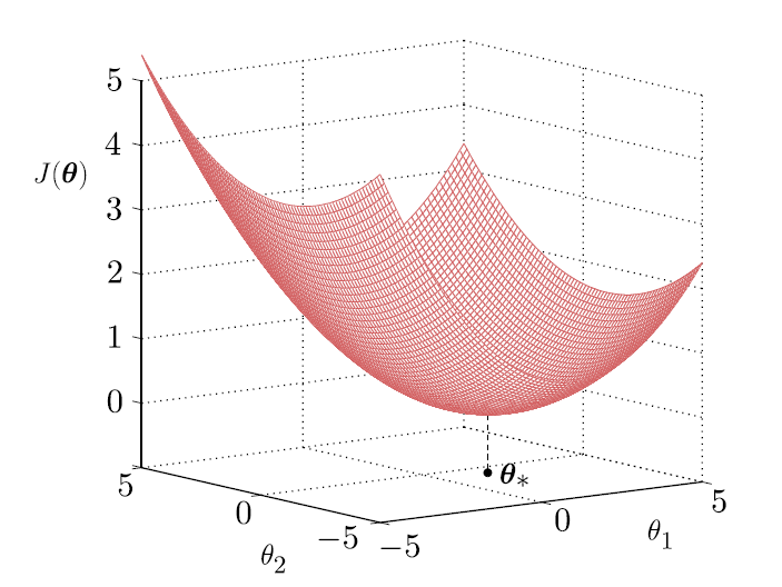
Neural nets will not be this kind.

3. A map of the math

The next figure is the course’s reminder of which math shows up where. Module 1 lives in the vector-calculus and optimization blocks. Later modules reuse the same objects (gradients, Hessians, inner products, eigenvalues) on new models.

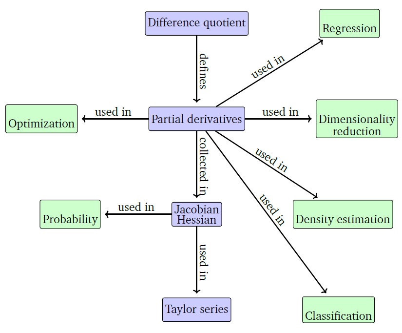
To minimize a smooth $J$ you need:

• a gradient (first derivatives) — when to stop, which way is downhill;
• a Hessian (second derivatives) — how curved the bowl is;
• later, constraints (Week 3) when $\mathit{\theta }$ is not free in ${ℝ}^l$.

The next two notes are those derivatives. Week 2 turns them into algorithms.

4. Practice

1. Why is the normal equation a calculus problem, not a programming problem?

2. In the auto-encoder example, what is $J$, and why does the chain rule appear?

3. If ${𝐗}^{\top }𝐗$ is not invertible, what did the data do, and what do you change before you invert?