2.2 Unconstrained Methods

Line search, steepest descent, momentum, and SGD.

These notes walk through the lecture slides. The original deck is unchanged; use (slides) on the course hub if you want that PDF.

The figures follow Deisenroth, Faisal, and Ong, Mathematics for Machine Learning.

1. Line search

Draw $x$ , predict $y_{p r e d}$ , score the mismatch with $J$ , take the gradient, and step against it.

Gradient step

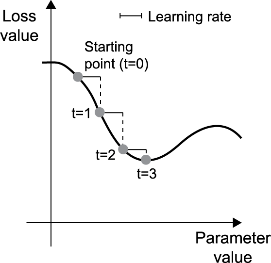
Almost every method in this note is

θ^{(k + 1)} = θ^{(k)} + α^{(k)} 𝐬^{(k)} .

Pick a direction $𝐬^{(k)}$ .
Pick a step $α^{(k)}$ (learning rate) that lowers $J (θ^{(k)} + α 𝐬^{(k)})$ in $α$ .
Take the step.

A direction is a descent direction when $𝐬^{⊤} \nabla J < 0$ . Steepest descent (gradient descent) uses $𝐬 = - \nabla J$ .

Following the negative gradient

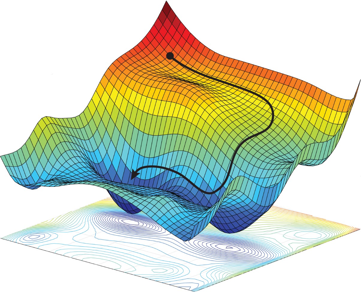
2. Why steepest descent zigzags

Steepest descent can be slow. The step length matters, and the asymptotic rate is worse than Newton-type methods. On a long thin valley the problem is poorly conditioned: $- \nabla J$ points into the walls, almost orthogonal to the short path to the min. Exact line search still hops.

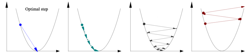
Well-conditioned versus poorly conditioned contours

See it on a quadratic. Let

J (θ) = \frac{1}{2} θ^{⊤} 𝐐 θ - C

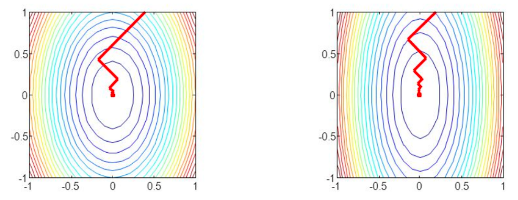
with $𝐐$ symmetric positive definite. Diagonalize $𝐐 = 𝐔 Λ 𝐔^{⊤}$ . In coordinates $𝐳 = 𝐔^{⊤} θ$ , minimizing $J$ is the same as minimizing $\sum_{i} λ_{i} z_{i}^{2}$ . In two dimensions the contours are ellipses

λ_{1} z_{1}^{2} + λ_{2} z_{2}^{2} = c .

The axis ratio is the condition number of $𝐐$ (largest over smallest eigenvalue). Large condition number: a long thin valley, tiny progress.

Slow zigzag on a poorly scaled bowl

3. Momentum

Remember the last step and refuse to turn on a dime (Rumelhart et al., 1986):

θ^{(k + 1)} = θ^{(k)} - α^{(k)} \nabla J (θ^{(k)}) + β Δ θ^{(k)},

Δ θ^{(k)} = θ^{(k)} - θ^{(k - 1)} = β Δ θ^{(k - 1)} - α^{(k - 1)} \nabla J (θ^{(k - 1)}),

with $β \in [0, 1]$ . A heavy ball in a valley: oscillations damp, progress along the floor improves. Noisy gradients benefit because the memory averages them. Stochastic approximations of $\nabla J$ are the usual case, not a special case.

4. SGD and mini-batches

If $J = \sum_{n = 1}^{N} J_{n}$ , batch gradient descent uses the full sum. That is expensive when $N$ is large and there is no closed form for $\nabla J$ .

SGD uses one term (or a random subset) as a noisy stand-in for $\nabla J$ . With a decaying step size, SGD converges almost surely to a local min under mild assumptions.

Mini-batch gradient descent sits in between: a random subset, not one row and not all $N$ . Still an unbiased estimate of the true gradient. Cheaper than batch, less noisy than one-row SGD.

Batch, SGD, and mini-batch paths

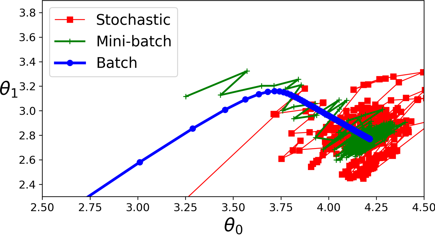
Why accept an approximate gradient?

Mini-batch	What you buy	What you pay
Large	Accurate $\nabla J$ , stable steps, fast matrix kernels	Each step is expensive; easy to sit in a sharp hole
Small	Cheap steps; noise can leave a bad local min; often enough for generalization	Higher variance in the updates

Memory and wall-clock are the practical reasons. Mini-batch size is a sample size for an empirical mean.

5. Practice

What does a large condition number do to steepest descent?
Write the descent test $𝐬^{⊤} \nabla J < 0$ in words. Why does $𝐬 = - \nabla J$ pass it whenever you are not already at a critical point?
Name one reason to prefer a small mini-batch over a large one, and one reason for the opposite.

Ahmad Mousavi

1. Line search

2. Why steepest descent zigzags

3. Momentum

4. SGD and mini-batches

5. Practice