8.2 Tensor Decomposition Algorithms

CP, Tucker, and how the factors are computed.

These notes walk through the lecture slides. The original deck is unchanged; use (slides) on the course hub if you want that PDF.

Figures and notes follow Introduction to Tensor Decompositions and their Applications in Machine Learning.

1. Tucker decomposition

Tucker writes a tensor as a core tensor plus a factor matrix per mode. It is a higher-order PCA.

Core tensor. A compressed version of the original: the essential interactions, in a smaller array.

Factor matrices. Principal components in that mode. Multiply them with the core to stretch back to the original sizes.

2. Why higher-order PCA?

PCA decomposes a matrix into orthogonal components that capture variance. Tucker does the same for a tensor: a core, and matrices that capture variance along each mode.

PCA reduces matrix dimension by keeping the important components. Tucker reduces tensor dimension by keeping the important interactions. That is the analysis and visualization move for multiway data.

3. Practical benefits

Compression. Choose a core smaller than $𝒳$ . Less storage, cheaper arithmetic.

Interpretability. Each column of a factor matrix is a principal component along that mode.

Flexibility. You choose the core size, so you choose how much you compress versus how much detail you keep. Other decompositions are less free here.

Picture the core as a small dense block of interactions, and each factor matrix as axes that stretch or compress that block back toward the data.

4. Problem formulation

For $𝒳 \in ℝ^{I \times J \times K}$ , find $𝒢 \in ℝ^{P \times Q \times R}$ , $𝐀 \in ℝ^{I \times P}$ , $𝐁 \in ℝ^{J \times Q}$ , $𝐂 \in ℝ^{K \times R}$ solving

{min}_{\hat{𝒳}} ‖ 𝒳 - \hat{𝒳} ‖ with \hat{𝒳} = \sum_{p = 1}^{P} \sum_{q = 1}^{Q} \sum_{r = 1}^{R} g_{p q r} 𝐚_{p} ⊚ 𝐛_{q} ⊚ 𝐜_{r} = 𝒢 \times_{1} 𝐀 \times_{2} 𝐁 \times_{3} 𝐂 .

Tucker decomposition: core and three factor matrices

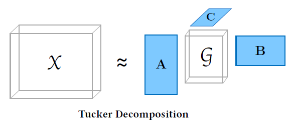
$𝒢$ is the core: how, and how much, elements interact.
$𝐀$ , $𝐁$ , $𝐂$ are the principal components in each mode.
If $P < I$ , $Q < J$ , $R < K$ , you compress: $𝒢$ is the compressed $𝒳$ .

Matricized form ( $\otimes$ is Kronecker):

{\hat{X}}_{(1)} = 𝐀 G_{(1)} (𝐂 \otimes 𝐁)^{⊤},

{\hat{X}}_{(2)} = 𝐁 G_{(1)} (𝐂 \otimes 𝐀)^{⊤},

{\hat{X}}_{(3)} = 𝐂 G_{(1)} (𝐁 \otimes 𝐀)^{⊤} .

$N$ -way:

\hat{𝒳} = \sum_{r_{1} = 1}^{R_{1}} \dots \sum_{r_{N} = 1}^{R_{N}} g_{r_{1} \dots r_{N}} 𝐚_{i_{1} r_{1}}^{(1)} ⊚ \dots ⊚ 𝐚_{i_{N} r_{N}}^{(N)} = 𝒢 \times_{1} 𝐀^{(1)} \times_{2} \dots \times_{N} 𝐀^{(N)},

{\hat{X}}_{(n)} = 𝐀^{(n)} G_{(n)} (𝐀^{(N)} \otimes \dots \otimes 𝐀^{(n + 1)} \otimes 𝐀^{(n - 1)} \otimes \dots \otimes 𝐀^{(1)})^{⊤} .

5. $n$ -rank

Before computing Tucker, you need $n$ -rank.

The $n$ -rank of $𝒳 \in ℝ^{I_{1} \times \dots \times I_{N}}$ is the column rank of the $n$ th unfolding $X_{(n)}$ , written ${rank}_{n} (𝒳)$ .

This is not the tensor rank of the previous note.

6. Higher-order SVD (HOSVD)

For a given $𝒳$ there is an exact Tucker decomposition of rank $(R_{1}, \dots, R_{N})$ with $R_{n} = {rank}_{n} (𝒳)$ . That factorization is HOSVD.

The idea: in each mode $n$ , find the components that best capture variation in that mode alone, ignoring the others for that step. PCA, one unfolding at a time.

HOSVD $(𝒳; R_{1}, \dots, R_{N})$ :

For $n = 1, \dots, N$ : set $𝐀^{(n)}$ to the $R_{n}$ leading left singular vectors of $X_{(n)}$ .
Core:

𝒢 = 𝒳 \times_{1} 𝐀^{(1) ⊤} \times_{2} \dots \times_{N} 𝐀^{(N) ⊤} .

Return $𝒢, 𝐀^{(1)}, \dots, 𝐀^{(N)}$ .

7. Limitations of Tucker

Cost. Factor matrices plus core are expensive for large tensors and high ranks.
Memory. The core and the factors can be large.
Initialization. Quality can depend on the starting factors; optimality is not guaranteed.

8. Canonical polyadic decomposition (CPD)

An alternative: write the tensor as a sum of a finite number of rank-1 tensors. CPD comes from CANDECOMP (canonical decomposition) and PARAFAC (parallel factors).

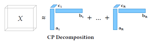
Canonical polyadic decomposition as a sum of rank-1 terms

	Tucker	CPD
Flexibility	Different ranks per mode; complex interactions	Rank-1 sum; simpler structure
Interpretability	Core shows how modes interact	Factor matrices as patterns in each mode
Compression / scale	Can compress well when interactions are complex	Cheaper; often scales better on large or high-order data

Practice

In Tucker, what does the core tensor store that a CPD sum of rank-1 terms does not?
How does HOSVD choose each factor matrix $𝐀^{(n)}$ ?
When might you prefer CPD to Tucker?

Ahmad Mousavi