5.3 Support Vector Machines

Margins, the dual, and the kernel trick.

These notes walk through the lecture slides. The original deck is unchanged; use (slides) on the course hub if you want that PDF.

The figures follow Deisenroth, Faisal, and Ong, Mathematics for Machine Learning, Theodoridis, and Géron, Hands-On Machine Learning.

1. The main idea

Think of open and filled circles as houses in two villages. A road between them should be as wide as possible and should demolish as few houses as possible. No sensible engineer picks the dash-dotted path in the figure.

A classifier should sit between the dense regions of the two classes, in a sparse belt, leaving the largest possible margin. That is the usual requirement for generalization: small error on points that were not in the training set.

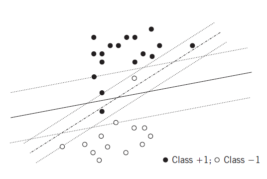
Maximum-margin road between two villages

2. Linearly separable classes

If the classes are linearly separable, infinitely many hyperplanes classify the training set with zero error. From that family one can always keep those that satisfy

y_{n} (θ^{⊤} x_{n} + θ_{0}) \geq 1, n = 1, \dots, N .

The SVM picks the one with smallest norm:

\underset{θ \in ℝ^{l}}{minimize} & \frac{‖ θ ‖^{2}}{2} subject to & y_{n} (θ^{⊤} x_{n} + θ_{0}) \geq 1, n = 1, \dots, N .

$‖ θ ‖$ is tied directly to the margin.

3. Primal, dual, and support vectors

The constrained problem is the primal. It has a dual. In general the dual only lower-bounds the primal; under convexity (and regularity of the constraints) the values match. SVM meets those conditions, so you may solve either.

The Lagrangian is

ℒ (θ, θ_{0}, λ) = \frac{1}{2} ‖ θ ‖^{2} - \sum_{n = 1}^{N} λ_{n} (y_{n} (θ^{⊤} x_{n} + θ_{0}) - 1) .

KKT stationarity gives

\nabla_{θ} ℒ = 0 \Rightarrow \hat{θ} = \sum_{n = 1}^{N} λ_{n} y_{n} x_{n} .

and

\nabla_{θ_{0}} ℒ = 0 \Rightarrow \sum_{n = 1}^{N} λ_{n} y_{n} = 0, λ_{n} (y_{n} (θ^{⊤} x_{n} + θ_{0}) - 1) = 0, λ_{n} \geq 0 .

Plug that expansion into $ℒ$ and solve the dual with a quadratic program:

\underset{λ}{minimize} & \frac{1}{2} \sum_{n = 1}^{N} \sum_{m = 1}^{N} λ_{n} λ_{m} y_{n} y_{m} x_{n}^{⊤} x_{m} - \sum_{n = 1}^{N} λ_{n} subject to & λ_{n} \geq 0, \sum_{n = 1}^{N} λ_{n} y_{n} = 0 .

With a dual solution $\hat{λ}$ ,

\hat{θ} = \sum_{n = 1}^{N_{s}} λ_{n} y_{n} x_{n},

where $N_{s}$ is the number of nonzero multipliers. Only points that meet the inequality as an equality, $y_{n} (θ^{⊤} x_{n} + θ_{0}) = 1$ , have $λ_{n} \neq 0$ . Those points are the support vectors. Recover ${\hat{θ}}_{0}$ from any such equality.

4. Notes

The SVM solution is unique: the cost is strictly convex.
The dual is usually faster than the primal.
The dual is what makes the kernel trick possible. In an RKHS the predictor is

\hat{y} (x) = \sum_{n = 1}^{N_{s}} λ_{n} y_{n} κ (x, x_{n}) + θ_{0} .

5. Non-separable classes

When the classes overlap, allow slack:

\underset{θ \in ℝ^{l}}{minimize} & \frac{‖ θ ‖^{2}}{2} + C \sum_{n = 1}^{N} ξ_{n} subject to & y_{n} (θ^{⊤} x_{n} + θ_{0}) \geq 1 - ξ_{n}, ξ_{n} \geq 0 .

A margin error is $y_{n} (θ^{⊤} x_{n} + θ_{0}) < 1$ , i.e. $ξ_{n} > 0$ . If $ξ_{n} = 0$ that point does not add to the cost. The optimizer tries to drive as many $ξ_{n}$ as possible to zero.

The user parameter $C$ trades the two terms. Large $C$ : a small margin, fewer margin errors. Small $C$ : the opposite.

6. Choice of hyper-parameters

$C$ is almost always chosen by cross-validation on held-out data.

The other choice is the kernel. Different kernels, different performance. A Gaussian kernel needs enough training points to fill the input space, because $κ (x, x_{n})$ matches $x$ to the stored point $x_{n}$ . Training-set size matters.

Kernel	Formula	Typical use
Linear	$κ (x, x^{'}) = x^{⊤} x^{'}$	Linearly separable data, or many features relative to $N$
Polynomial	$κ (x, x^{'}) = (x^{⊤} x^{'} + c)^{d}$	Polynomial-shaped boundaries (e.g. some image tasks)
Gaussian RBF	$κ (x, x^{'}) = \exp (- ‖ x - x^{'} ‖^{2} / (2 σ^{2}))$	Complex nonlinear relations
Sigmoid	$κ (x, x^{'}) = \tanh (α x^{⊤} x^{'} + c)$	Periodic or sigmoid-like relations (e.g. some time series)

7. Practice

Where do the support vectors appear in the SVM dual?
What does a large $C$ do to the margin and to margin errors?
Why does the dual make the kernel trick possible?

Ahmad Mousavi