4.1 Motivation for Sparsity-Aware Learning

Why we want models that can set coefficients to zero.

These notes walk through the lecture slides. The original deck is unchanged; use (slides) on the course hub if you want that PDF.

The figures follow Deisenroth, Faisal, and Ong, Mathematics for Machine Learning, and Theodoridis, Machine Learning: A Bayesian and Optimization Perspective.

1. Bias-variance trade-off

A simple linear model is

y = θ_{0} + θ_{1} x_{1} + θ_{2} x_{2} + \dots + θ_{l} x_{l} + ϵ .

Plain least squares is not the only way to estimate $θ$ . The goal of this module is better accuracy and better interpretability.

Regime	What least squares does
$N ≫ l$ , roughly linear	Low variance, low bias
$N > l$ but not by much	High variance; a small change in the training rows can swing the coefficients; overfitting
$l > N$	No unique least-squares estimate; variance is “infinite”

As the model gets more flexible, interpretability usually falls. Irrelevant columns add complexity. Setting some coefficients exactly to zero would drop those variables.

Solution. Constrain or shrink the coefficients: give up a little bias to cut variance, and predictions improve.

2. Compressed sensing

Compressed sensing (CS) tries to acquire as few samples as possible, as long as those samples still encode a compressed representation of the signal.

Compressed sensing

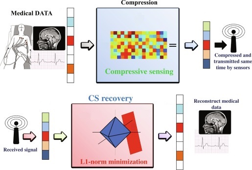
Let $𝐗 \in ℝ^{N \times l}$ be a sensing matrix applied to an unknown signal $s \in ℝ^{l}$ to get observations $y \in ℝ^{N}$ . Let $Ψ$ be a dictionary in which $s$ has a sparse representation

s = Ψ θ .

From $y = 𝐗 s$ one gets $y = 𝐗 Ψ θ$ . Given $𝐗$ and $Ψ$ (or the product $𝐗 Ψ$ ), one can recover $\hat{s}$ by an $ℓ_{1}$ program if at most $k$ coordinates of $θ$ are nonzero.

The linear system is under-determined, so it has an infinite number of solutions in general. The extra fact is that the true model is sparse: only a few coordinates are nonzero.

3. The $ℓ_{0}$ -norm

The $ℓ_{0}$ -“norm” counts nonzero coordinates. That is the most direct sparsity measure.

Comparing <math xmlns= ℓp norms" src="files/graphics/4.1-sparsity-motivation/norms.png" />

It is not usable as a training penalty: it is not differentiable, and optimizing it is NP-hard. Other $ℓ_{p}$ with $p < 1$ are non-convex, which is also a hard optimization problem. Later notes use $ℓ_{1}$ and $ℓ_{2}$ instead.

4. Practical examples

NLP. Most words in a document never appear, or appear once. A bag-of-words vector is sparse: one coordinate per vocabulary word, mostly zeros.
Image processing. Many pixels are background. Keeping only the useful features or regions gives a sparse representation, which is cheaper to store and to compute with.

5. Emerging applications

Medical imaging. Sparse MRI aims to reconstruct from fewer measurements, which shortens scans.
Signal processing. Compressive sensing for denoising and reconstruction recovers a sparse signal from undersampled measurements.
Recommendation. User–item matrices are sparse. Sparsity-aware methods can still suggest items when the history is thin (the cold-start setting).

6. Practice

In which regime is the least-squares variance “infinite,” and why?
Why is the $ℓ_{0}$ -norm a natural sparsity penalty, and why do we not optimize it directly?
What extra information lets compressed sensing pick one solution from an under-determined system?

Ahmad Mousavi