4.2 Ridge Regression

Shrink coefficients with an L2 penalty.

These notes walk through the lecture slides. The original deck is unchanged; use (slides) on the course hub if you want that PDF.

The figures follow Deisenroth, Faisal, and Ong, Mathematics for Machine Learning, and Theodoridis, Machine Learning: A Bayesian and Optimization Perspective.

1. Shrinkage methods

Among the $ℓ_{p}$ -norms with $p \geq 1$ , only $ℓ_{1}$ treats small coordinates with any respect. The others squeeze small values further and spend their attention on large ones.

Regularization is also there to make an estimator easier to interpret.

Least squares fits $θ_{0}, θ_{1}, \dots, θ_{l}$ by

\sum_{n = 1}^{N} (y_{n} - θ_{0} - \sum_{j = 1}^{l} θ_{j} x_{j})^{2} .

Ridge instead minimizes

\sum_{n = 1}^{N} (y_{n} - θ_{0} - \sum_{j = 1}^{l} θ_{j} x_{j})^{2} + λ \sum_{j = 1}^{l} θ_{j}^{2},

with hyper-parameter $λ \geq 0$ .

2. What $λ$ does

The penalty $λ \sum_{j = 1}^{l} θ_{j}^{2}$ forces the fit to keep the coefficients small. Add it only while training. Evaluate the trained model with the unregularized metric.

$λ$	Effect
$λ = 0$	Ridge is ordinary least squares
$λ \to \infty$	Ridge coefficients approach zero (they do not hit zero for finite $λ$ )

The penalty hits $θ_{1}, \dots, θ_{l}$ , not $θ_{0}$ . If every column of $𝐗 \in ℝ^{N \times l}$ is centered,

{\hat{θ}}_{0} = \bar{y} = \sum_{n = 1}^{N} y_{n} / N .

3. Geometry

Ridge geometry: ellipse and circle

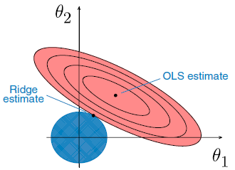
For $l = 2$ the ridge constraint is a circle

θ_{1}^{2} + θ_{2}^{2} \leq t,

where $\sqrt{t}$ is the radius. The RSS contours are ellipses. The ridge estimate is the point where the ellipse and the circle touch.

$λ = 0$ : you only shrink the ellipse (inner ellipses have smaller RSS). Highly correlated features make that geometry unpleasant.
Small $λ$ : more variance, less bias. Large $λ$ : some bias, less variance.

4. The closed form

J (θ) = (𝐲 - 𝐗 θ)^{⊤} (𝐲 - 𝐗 θ) + λ θ^{⊤} θ .

Expand:

J (θ) = 𝐲^{⊤} 𝐲 - 𝐲^{⊤} 𝐗 θ - θ^{⊤} 𝐗^{⊤} 𝐲 + θ^{⊤} 𝐗^{⊤} 𝐗 θ + λ θ^{⊤} θ .

Set the derivative to zero:

\frac{\partial J (θ)}{\partial θ} = - 2 𝐗^{⊤} 𝐲 + 2 𝐗^{⊤} 𝐗 θ + 2 λ θ = 0 .

Then

(𝐗^{⊤} 𝐗 + λ 𝐈) θ = 𝐗^{⊤} 𝐲,

{\hat{θ}}_{R} = (𝐗^{⊤} 𝐗 + λ 𝐈)^{- 1} 𝐗^{⊤} 𝐲 .

5. Comments

Ridge gives accurate predictions and reduced variance.
Penalizing coefficient size controls overfitting: the model is less free to memorize noise.
Ridge is the usual tool for multicollinearity. Shrinking correlated coefficients stabilizes the estimates.

6. Computational complexity

You can use the closed form or gradient descent, as with linear regression. The closed form inverts an $l \times l$ matrix (Cholesky and friends). That gets slow when the number of features is large. If there are too many features, or too many rows to fit in memory, use gradient descent.

7. Practice

Why can ridge shrink coefficients but not set them to zero?
What happens as $λ \to \infty$ , and which coefficient is never penalized?
Why does adding $λ 𝐈$ help when columns of $𝐗$ are highly correlated?

Ahmad Mousavi