6.3 Special Considerations for PCA

Centering, scaling, and how many components to keep.

These notes walk through the lecture slides. The original deck is unchanged; use (slides) on the course hub if you want that PDF.

Figures and notes follow Deisenroth, Faisal, and Ong, Mathematics for Machine Learning; Theodoridis; and Géron.

1. PCA and singular value decomposition (SVD)

Eigendecomposition. From the covariance $𝐒 = \frac{1}{N} \sum_{n = 1}^{N} x_{n} x_{n}^{⊤}$ , compute eigenvalues $λ_{i}$ and eigenvectors $u_{i}$ . The $u_{i}$ are the principal components. Each $λ_{i}$ is the variance along that component.

SVD. Factor the centered data matrix: $𝐗 = 𝐔 Σ 𝐕^{⊤}$ . The right singular vectors $𝐕$ are the principal components. The singular values on the diagonal of $Σ$ are the square roots of the eigenvalues of $𝐗^{⊤} 𝐗$ .

The two routes agree. That is the link between the maximum-variance view of PCA and the SVD of $𝐗$ .

2. PCA and low-rank approximations

Because $\hat{𝐗}$ is the best rank- $m$ approximation of $𝐗$ in the Frobenius sense,

‖ \hat{𝐗} - 𝐗 ‖_{F}^{2} = \sum_{n = 1}^{N} ‖ {\hat{x}}_{n} - x_{n} ‖^{2}

is minimum.

So PCA also minimizes the sum of squared reconstruction errors. The same components that maximize variance are the ones that keep as much of the original points as an $m$ -dimensional picture can.

3. Latent variable perspective

So far PCA had no probabilistic model: maximum variance and projection only. A probabilistic model would:

come with a likelihood, so noise in the observations is explicit;
allow Bayesian model comparison via the marginal likelihood;
treat PCA as a generative model (simulate new data);
make connections to related algorithms straightforward;
handle dimensions missing at random by Bayes;
give a notion of how novel a new point is;
extend cleanly, e.g. to a mixture of PCA models;
recover the PCA of the earlier sections as a special case;
allow a fully Bayesian treatment by integrating out parameters.

4. History of probabilistic PCA

A continuous latent $z \in ℝ^{M}$ lets you write PCA as a probabilistic latent-variable model. Tipping and Bishop (1999) called this probabilistic PCA (PPCA). It addresses most of the list above. Ordinary PCA — maximize projected variance, or minimize reconstruction error — is maximum likelihood in the noise-free limit.

5. The PPCA model

Assume a continuous latent $z \in ℝ^{M}$ with standard-normal prior $p (z) = 𝒩 (0, 𝐈)$ , and a linear map to the observation $x$ :

x = B z + μ + ϵ \in ℝ^{D},

where $ϵ ~ 𝒩 (0, σ^{2} 𝐈)$ is Gaussian observation noise, $B \in ℝ^{D \times M}$ , and $μ \in ℝ^{D}$ . The conditional is

p (x ∣ z; B, μ, σ^{2}) = 𝒩 (x ∣ B z + μ, σ^{2} 𝐈) .

The generative process:

z_{n} ~ 𝒩 (z ∣ 0, 𝐈)

and

x_{n} ∣ z_{n} ~ 𝒩 (x ∣ B z_{n} + μ, σ^{2} 𝐈) .

To draw a typical point, use ancestral sampling: first $z_{n} ~ p (z)$ , then $x_{n} ~ p (x ∣ z_{n}; B, μ, σ^{2})$ .

The joint is

p (x, z ∣ B, μ, σ^{2}) = p (x ∣ z, B, μ, σ^{2}) p (z) .

6. An illustration of PPCA

Blue dots: two-dimensional PCA latents for MNIST digits “8”. Query any $z_{*}$ in that plane and generate ${\tilde{x}}_{*} = B z_{*}$ (here $μ = 0$ and identity covariance). The image looks like an “8”.

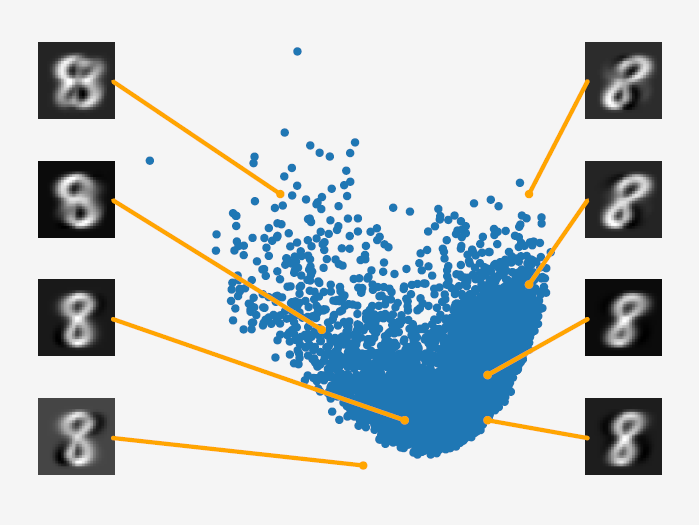
PPCA latent space and generated eights

Eight generated images sit with their latent coordinates. Where you query the latent plane changes shape, rotation, size.

Practice

In the SVD view of PCA, which factor of $𝐗 = 𝐔 Σ 𝐕^{⊤}$ holds the principal components?
Besides maximizing variance, what reconstruction quantity does a rank- $m$ PCA minimize?
In PPCA, what extra random object appears that ordinary PCA never named, and what prior does it get?

Ahmad Mousavi