7.3 Independent Vector Analysis

Independent components that stay aligned across datasets.

These notes walk through the lecture slides. The original deck is unchanged; use (slides) on the course hub if you want that PDF.

Figures and notes follow Diversity in Independent Component and Vector Analyses and Anderson, Development of ICA and IVA Algorithms.

1. Latent variable methods

For matrix factorization, write observations $𝐗 \in ℝ^{P \times V}$ as $𝐗 = 𝐁 𝐂$ , with latent matrix $𝐂 \in ℝ^{M \times V}$ .

Blind source separation as a factorization

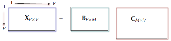
A typical cost:

{min}_{𝐁, 𝐂} ‖ 𝐗 - 𝐁 𝐂 ‖_{p}^{2} + λ_{1} \sum_{m = 1}^{M} h (𝐛_{m}) + λ_{2} \sum_{v = 1}^{V} g (𝐜_{v}) .

2. Independent component analysis (ICA)

ICA (1980s–90s) separates a multivariate signal into sources. Hérault and Jutten, 1985.

The cocktail party picture: several people talk at once; several microphones hear mixtures; recover each voice.

Cocktail party and ICA

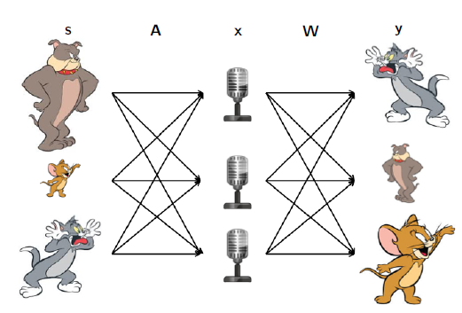
The model:

𝐱 = 𝐀 𝐬,

with observations $𝐱$ and latent sources $𝐬$ mixed by $𝐀$ .

ICA mixing model

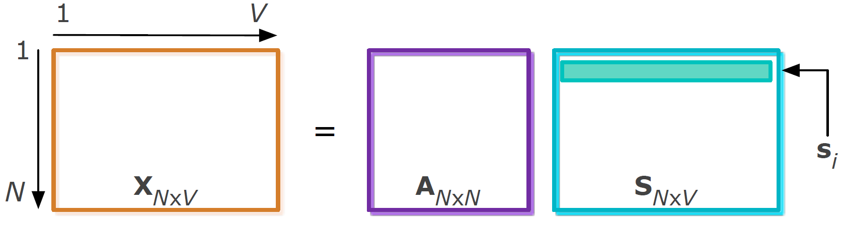
ICA can identify the sources up to scale and permutation if the sources are statistically independent.

3. The ICA objective

One ICA objective is mutual information among the estimated sources: the KL distance between the joint source density and the product of the marginals. With $p_{𝐬} (𝐖 𝐱) = p_{𝐱} (𝐱) | det (𝐖) |^{- 1}$ ,

J_{I C A} (𝐖) & = 𝔼 \{- \log [\frac{p_{s_{1}} (y_{1}) p_{s_{2}} (y_{2}) \dots p_{s_{N}} (y_{N})}{p_{s_{1} s_{2} \dots s_{N}} (y_{1}, y_{2}, \dots, y_{N})}] \} & = 𝔼 \{- \sum_{n = 1}^{N} \log p_{s_{n}} (y_{n}) \} + 𝔼 {\log p_{𝐬} (𝐲)} & = \sum_{n = 1}^{N} H (y_{n}) - H (𝐲) & = \sum_{n = 1}^{N} H (y_{n}) - \log | det (𝐖) | - H (𝐱),

where $H (y_{n})$ and $H (𝐱)$ are the differential entropies of the source estimates and of the mixtures.

4. ICA algorithms

The score function can be estimated in three styles.

Parametric. FastICA, EFICA, Infomax. A fixed nonlinearity or a fixed source density. Cheap. Separation suffers when the true sources are far from that model.

Nonparametric. RADICAL uses entropy estimates. Parameter choices are awkward. Cost grows with sample size.

Semi-parametric. ICA-EBM and ICA-EMK. Flexible density matching via measuring functions from the maximum-entropy principle. Broad PDFs; sometimes expensive.

5. Independent vector analysis (IVA)

In practice you often have several data sets that depend on one another.

IVA model across data sets

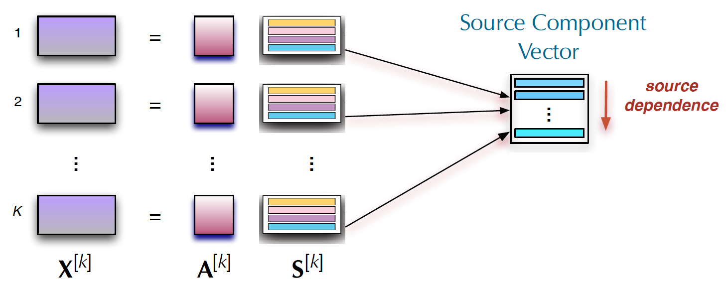
IVA uses a source component vector (SCV): the $n$ th source from each of the $K$ data sets, stacked,

𝐬_{n} = [s_{n}^{[1]}, \dots, s_{n}^{[K]}]^{⊤},

a $K$ -dimensional random vector.

Goal. Estimate $K$ demixing matrices so that $𝐲^{[k]} = 𝐖^{[k]} 𝐱^{[k]}$ and each SCV is maximally independent of the other SCVs.

The noiseless model, i.i.d. samples, is ICA repeated $K$ times,

𝐱^{[k]} = 𝐀^{[k]} 𝐬^{[k]}, k = 1, \dots, K,

with invertible $𝐀^{[k]} \in ℝ^{N \times N}$ and $𝐬^{[k]} = [s_{1}^{[k]}, \dots, s_{N}^{[k]}]^{⊤}$ . Within each $𝐬^{[k]}$ the components are independent. Across data sets, corresponding components of $𝐬^{[k]}$ may depend.

6. The IVA objective

Maximum likelihood again, but the parameter is a set of demixing matrices $𝐖^{[1]}, \dots, 𝐖^{[K]}$ , packed as a three-way array $𝒲 \in ℝ^{N \times N \times K}$ . Mutual information:

J_{I V A} (𝒲) = \sum_{n = 1}^{N} H (𝐲_{n}) - \sum_{k = 1}^{K} \log | det (𝐖^{[k]}) | - H (𝐱^{[1]}, \dots, 𝐱^{[K]}),

where $H (𝐲_{n})$ is the entropy of the $n$ th SCV. The last term is constant.

7. Gradient and updates

Differentiating in each demixing matrix, as in ICA,

\frac{\partial J_{I V A} (𝒲)}{\partial 𝐖^{[k]}} = 𝔼 \{ϕ^{[k]} (𝐱^{[k]})^{⊤} \} - (𝐖^{[k]})^{- ⊤},

with

ϕ^{[k]} = - [\frac{\partial \log p_{s_{1}} (y_{1})}{\partial y_{1}^{[k]}}, \dots, \frac{\partial \log p_{s_{N}} (y_{N})}{\partial y_{N}^{[k]}}]^{⊤} .

Each of the $K$ matrices steps by

(𝐖^{[k]})^{n e w} \leftarrow (𝐖^{[k]})^{o l d} - γ \frac{\partial J_{I V A} (𝒲)}{\partial 𝐖^{[k]}},

with step size $γ$ .

8. IVA algorithms

Most IVA methods estimate the score parametrically.

Method	Assumption
IVA-L (Laplacian)	Higher-order statistics; Laplacian SCVs
IVA-G (Gaussian)	Linear dependence only, no HOS; Gaussian sources. Gradient simplifies; Hessian positive definite; Newton-type updates become practical
IVA-GGD / IVA-A-GGD	Second- and higher-order statistics; multivariate generalized Gaussian. Gaussian and Laplacian are special cases
IVA-M-EMK	Multivariate entropy maximization with kernels, when the matching multidimensional PDF matters. Can be cheaper as $K$ and $N$ grow

Practice

What extra assumption does IVA add on top of ICA?
ICA identifies sources only up to two ambiguities. What are they, and what statistical assumption buys uniqueness?
What is a source component vector, and what does IVA want of distinct SCVs?

Ahmad Mousavi