6.1 Introduction to PCA

DATA 442/642 · Week 6 · PDF · Slides

Directions of largest variance, and the covariance eigenproblem.

These notes walk through the lecture slides. The original deck is unchanged; use (slides) on the course hub if you want that PDF.

Figures and notes follow Deisenroth, Faisal, and Ong, Mathematics for Machine Learning; Theodoridis; and Géron.

1. Principal Component Analysis (PCA)

PCA is the usual dimensionality reduction algorithm. It finds the hyperplane that maximizes the variance of the data, then projects onto that hyperplane.

Pearson (1901) introduced the idea as the principal axis theorem. Hotelling (1930s) gave the modern name. It began as a statistics tool for data analysis and dimension reduction.

2. Preserving the variance

You have to choose the hyperplane before you project.

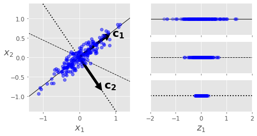
A 2D set, three candidate axes (one-dimensional hyperplanes). The right panel is the projection onto each.

• The solid line keeps the most variance.
• The dotted line keeps almost none.
• The dashed line sits in between.

The axis that preserves maximum variance loses the least information. That is the idea behind PCA.

3. Principal components

The working assumption, here and in other dimension-reduction methods: the observations come from a process driven by a relatively small number of latent (unobserved) variables. The goal is to recover that structure.

PCA finds the axis of largest variance in the training set (the solid line above). Then a second axis, orthogonal to the first, that takes the largest remaining variance. In higher dimension it keeps going: a third orthogonal to both, a fourth, as many axes as the original dimension.

The direction of a PC is not stable. Perturb the training set a little and some new PCs may point the opposite way — still on the same axes. A pair of PCs can rotate or swap; the plane they span usually stays.

4. Maximum variance perspective

Centered observations ${\mathit{x}}_1,\dots ,{\mathit{x}}_N$ in ${ℝ}^l$ (subtract the mean if needed). PCA looks for a subspace of dimension $m\le l$ so that projected variance is maximized. That subspace is spanned by $m$ mutually orthogonal principal axes.

Start with $m=1$. Let ${\mathit{u}}_1$ be the axis. Projected variance is

where

is the biased sample covariance.

Directions only, so take $\mathit{u}$ of unit length:

Lagrangian:

Set the gradient to zero:

The principal direction is an eigenvector of the sample covariance. Plug $𝐒\mathit{u}=\lambda \mathit{u}$ back into ${\mathit{u}}^{\top }𝐒\mathit{u}$ with ${\mathit{u}}^{\top }\mathit{u}=1$:

Variance is maximized when ${\mathit{u}}_1$ is the eigenvector for the largest eigenvalue ${\lambda }_1$. $𝐒$ is symmetric positive semidefinite, so the eigenvalues are real and nonnegative. If $𝐒$ is invertible (hence $N>l$) they are positive. Assume they are distinct: ${\lambda }_1>{\lambda }_2>\dots >{\lambda }_l>0$.

The second PC is (a) orthogonal to ${\mathit{u}}_1$ and (b) maximizes remaining variance. It is the eigenvector for ${\lambda }_2$. Continue until $m$ axes: the eigenvectors for the $m$ largest eigenvalues.

5. Practical aspects

Eigenvectors show up in other matrix decompositions too.

You can write eigenvalues as roots of the characteristic polynomial. For matrices larger than $4\times 4$ there is no algebraic formula (Abel–Ruffini). Packages use iterative methods for eigenvalues and singular values.

Often you only want the first few eigenvectors. Computing a full eigendecomposition (or SVD) and throwing the rest away is wasteful. Iterative methods that target those few are cheaper. If you only need the first eigenvector, power iteration is efficient.

Practice

1. PCA maximizes variance. What matrix’s eigenvectors are you computing?

2. Why constrain ${\mathit{u}}^{\top }\mathit{u}=1$, and what does the multiplier $\lambda$ equal at the solution?

3. If you perturb the training set slightly, what about the principal components can flip, and what usually stays put?