2.1 Introduction to Optimization

DATA 442/642 · Week 2 · PDF · Slides

Cost functions, local versus global minima, convexity, and first- and second-order tests.

These notes walk through the lecture slides. The original deck is unchanged; use (slides) on the course hub if you want that PDF.

The figures follow Deisenroth, Faisal, and Ong, Mathematics for Machine Learning.

1. Training is optimization

Training a model is finding a good $\mathit{\theta }$. Good is whatever the cost (objective) $J$ says it is.

Write $J(\mathit{\theta }):S\to ℝ$ and solve

Usually $S={ℝ}^l$. This course always minimizes. Maximizing profit $P$ is minimizing $-P$.

2. Linear regression

Model $y={\mathit{\theta }}^{\top }𝐱+\epsilon$. Fit by minimizing mean squared error on $m$ training rows:

Each step that lowers $J$ shrinks residuals. Better $\mathit{\theta }$ on the training set is the hope that predictions on new $𝐱$ improve too. That hope is generalization; the math this week is the min.

3. Local versus global

A local minimum is lowest in a neighborhood: some $\epsilon >0$ such that $\Vert \mathit{\theta }-\widehat{\mathit{\theta }}\Vert <\epsilon$ implies $J(\widehat{\mathit{\theta }})\le J(\mathit{\theta })$. A global minimum is lowest on all of $S$.

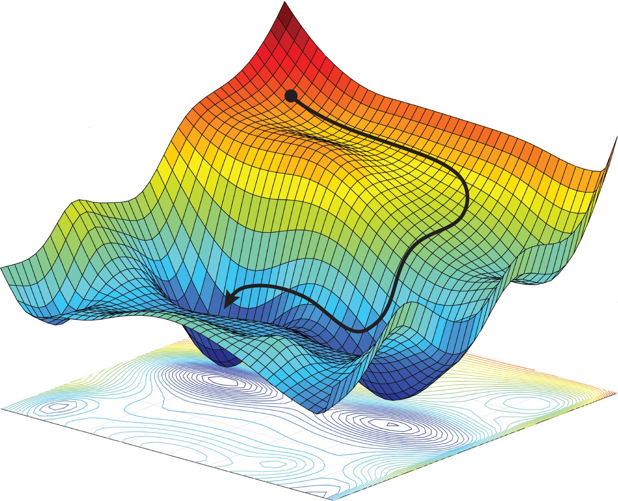
A valley on a hike is local. The lowest point in the whole range is global. Neural-net costs look like the landscape below. Many valleys. The one you land in need not be the lowest.

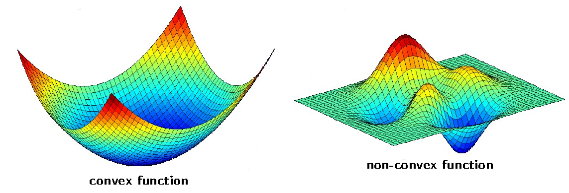
If $J$ is convex,

for all $\mathit{\theta },\mathit{\beta }\in S$ and all $t\in (0,1)$, then every local min is global.

Convex: gradient descent that reaches a local min has the global min. Nonconvex: you can stop in a valley that is not the bottom.

4. First- and second-order tests

First-order (necessary). At a local min of a smooth unconstrained $J$, $\nabla J(\widehat{\mathit{\theta }})=\mathbf{0}$. The slope is flat.

Second-order (sufficient). If that point also has Hessian ${\nabla }^{2}J(\widehat{\mathit{\theta }})$ positive definite, it is a local min.

A zero gradient is not enough: a saddle is flat and is not a min. Week 2’s algorithms either follow $-\nabla J$ or invert ${\nabla }^{2}J$.

5. Practice

1. When does a local minimum fail to be global?

2. Why does this course write every learning problem as a min, even when the story is “maximize likelihood”?

3. At a point with $\nabla J=\mathbf{0}$, what extra fact about ${\nabla }^{2}J$ lets you call it a local min rather than a saddle?