5.1 Hilbert Spaces

DATA 442/642 · Week 5 · PDF · Slides

Inner-product spaces as the setting for kernels.

These notes walk through the lecture slides. The original deck is unchanged; use (slides) on the course hub if you want that PDF.

The figures follow Deisenroth, Faisal, and Ong, Mathematics for Machine Learning, Theodoridis, and Géron, Hands-On Machine Learning.

1. Central idea

Many datasets live on a nonlinear set. One response is to map the inputs to a new space where the same task becomes linear. Choosing that map is not obvious.

Given pairs $(y_n,{\mathit{x}}_n)$ for $n=1,\dots ,N$, apply $\mathit{\varphi }:{ℝ}^l\to {ℝ}^K$ with $K\gg l$ so that the images $\mathit{\varphi }({\mathit{x}}_n)$ are linearly separable in ${ℝ}^K$.

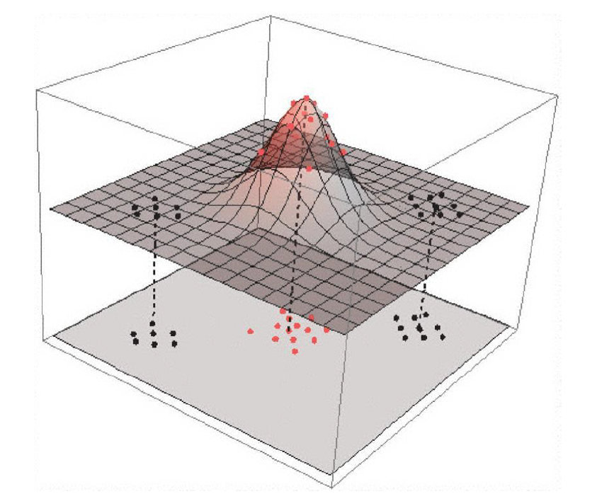
Points that cannot be separated by a line in the original plane can be separated by a plane after a nonlinear map into 3-space. You have embedded an $l$-dimensional manifold in a $K$-dimensional space so the two classes become linearly separable.

Working in that high-dimensional space is expensive: many parameters, computational cost, and a real risk of overfitting.

2. Kernels and RKHS

Instead of writing $\mathit{\varphi }$ and computing inner products of $\mathit{\varphi }({\mathit{x}}_i)$ and $\mathit{\varphi }({\mathit{x}}_j)$, define a similarity $\kappa ({\mathit{x}}_i,{\mathit{x}}_j)$. For a class of similarities called kernels, that function implicitly defines a feature map $\mathit{\varphi }$.

Let $ℍ$ be a Hilbert space of real-valued functions: an inner product, and completeness in the induced norm. $ℍ$ is a reproducing kernel Hilbert space (RKHS) if there is a kernel $\kappa :𝒳\times 𝒳\to ℝ$ such that every $f\in ℍ$ and every $\mathit{x}\in 𝒳$ satisfy $f(\mathit{x})=⟨f,\kappa (·,\mathit{x})⟩$. In this course, think $𝒳={ℝ}^l$ and $ℍ={ℝ}^K$.

Each kernel $\kappa$ has a unique RKHS (Aronszajn, 1950). The canonical feature map is $\mathit{\varphi }(\mathit{x})=\kappa (·,\mathit{x})$, and $ℍ$ is the feature space.

The kernel trick: for any two points,

Inner products in $ℍ$ become a function evaluation in the original low-dimensional space.

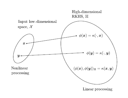
The nonlinear task in the original space is linear in the RKHS. In practice: (a) write the algorithm using only inner products in the original space, then (b) replace those inner products by kernel evaluations.

The matrix $𝐊\in {ℝ}^{N\times N}$ of those pairwise evaluations is the kernel matrix. Every kernel matrix is symmetric and positive semidefinite.

Choose the kernel (and its parameters) by nested cross-validation. The specific formula for $\kappa$ does not enter the derivation. After you have the predictor, you can swap kernels; each choice is a different nonlinearity.

3. Representer theorem

The representer theorem lets you optimize an empirical loss over a finite sample even when $f$ lives in a very high-dimensional (even infinite-dimensional) RKHS.

Theorem. Let $\Omega :[0,\infty )\to ℝ$ be strictly increasing, and let $ℒ:{ℝ}^2\to ℝ$ be any loss. Each minimizer $f\in ℍ$ of

has the form

with ${\theta }_n\in ℝ$.

To minimize $J$ you plug in that expansion and optimize only the finite list ${\theta }_1,\dots ,{\theta }_N$.

4. Practice

1. What does the kernel trick replace an inner product in $ℍ$ with?

2. Why is working with an explicit high-dimensional map $\mathit{\varphi }$ expensive?

3. What does the representer theorem say you may optimize instead of the function $f\in ℍ$?