11.1 Gaussian Mixture Models

Soft clusters as a mixture of Gaussians.

These notes walk through the lecture slides. The original deck is unchanged; use (slides) on the course hub if you want that PDF.

Figures and notes follow Géron, Hands-On Machine Learning; Deisenroth, Faisal, and Ong, Mathematics for Machine Learning; and Theodoridis.

1. Gaussian mixture models

A GMM says each row was drawn from a mixture of Gaussians whose parameters you do not know.

One Gaussian → one cluster. Clusters look like ellipsoids. They may differ in shape, size, density, and orientation.

Data from a mixture of Gaussians

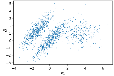
You see an instance. You do not see which Gaussian wrote it, and you do not know the parameters.

2. The generative story

For each $x_{i}$ , pick a cluster $z_{i}$ among $k$ clusters. The probability of cluster $j$ is its weight $ϕ_{j}$ :

P (z_{i} = j) = ϕ_{j} .

If $z_{i} = j$ , draw the location from that Gaussian:

x_{i} ~ 𝒩 (μ_{j}, Σ_{j}) .

So $𝐗$ comes from $k$ Gaussians, each with a weight $ϕ_{j}$ , a mean $μ_{j}$ , and a covariance $Σ_{j}$ . Collect those as $θ$ . The job is to estimate $θ$ from the observed $𝐗$ .

3. Log-likelihood

The log-likelihood is the log probability of the data and the latent cluster ids under $θ$ :

\log p (𝐗, 𝐙 ∣ θ) = \sum_{i = 1}^{n} \log p (x_{i}, z_{i} ∣ θ) = \sum_{i = 1}^{n} \log (\sum_{j = 1}^{k} ϕ_{j} 𝒩 (x_{i} ∣ μ_{j}, Σ_{j})) .

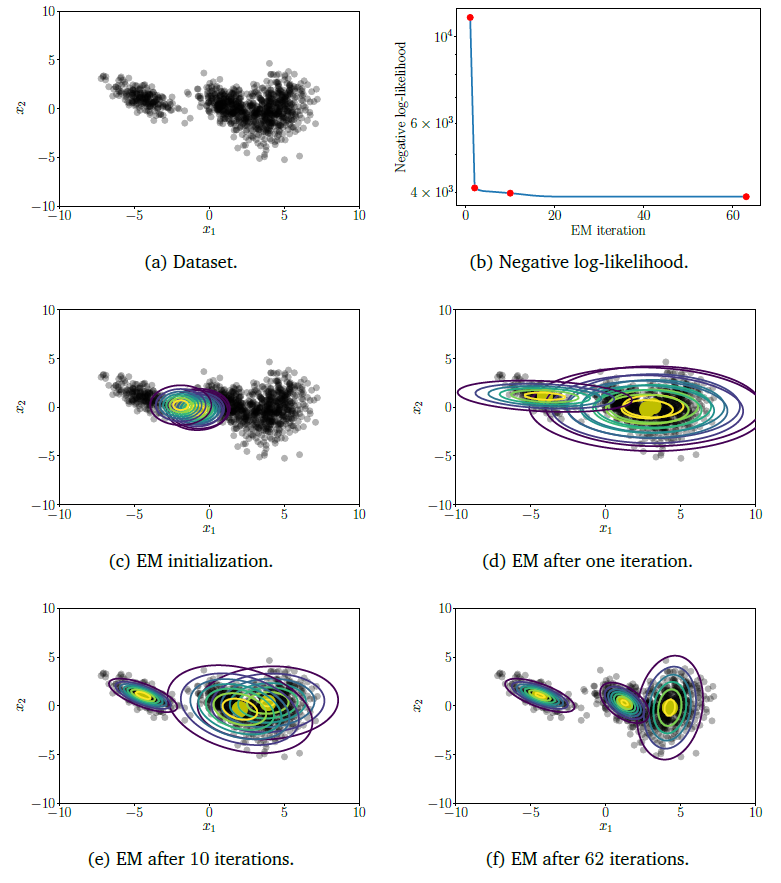
Maximize this in $θ$ . Expectation-maximization (EM) does it by alternating an E-step and an M-step until the likelihood stops moving.

4. Expectation-maximization

E-step. Soft assignment: probability that point $i$ came from cluster $j$ , given the current $θ^{(t)}$ :

γ^{(t)} (z_{i j}) = \frac{ϕ_{j}^{(t)} 𝒩 (x_{i} ∣ μ_{j}^{(t)}, Σ_{j}^{(t)})}{\sum_{j = 1}^{k} ϕ_{j}^{(t)} 𝒩 (x_{i} ∣ μ_{j}^{(t)}, Σ_{j}^{(t)})} .

M-step. Update means, covariances, and weights to fit those responsibilities.

Means:

μ_{j}^{(t + 1)} = \frac{\sum_{i = 1}^{n} γ^{(t)} (z_{i j}) x_{i}}{\sum_{i = 1}^{n} γ^{(t)} (z_{i j})} .

Covariances:

Σ_{j}^{(t + 1)} = \frac{\sum_{i = 1}^{n} γ^{(t)} (z_{i j}) (x_{i} - μ_{j}^{(t + 1)}) (x_{i} - μ_{j}^{(t + 1)})^{⊤}}{\sum_{i = 1}^{n} γ^{(t)} (z_{i j})} .

Weights:

ϕ_{j}^{(t + 1)} = \frac{\sum_{i = 1}^{n} γ^{(t)} (z_{i j})}{n} .

Repeat. Each pair of steps raises the likelihood a little. Stop when $θ$ barely changes.

EM iterating on a Gaussian mixture

5. Applications

Image segmentation. Color or texture. Soft membership helps on ambiguous pixels. Lighting and texture can vary; a mixture of Gaussians can still fit the intensities.

Anomaly detection. Model ordinary behavior as a mixture of Gaussians. Deviations are anomalies. Network traffic, transactions, sensors.

Speech. Model features such as Mel-frequency cepstral coefficients (MFCCs). The mixture captures how speech sounds vary; that is a classic acoustic model.

6. Practical notes

Initialization. Random, $k$ -means then covariances, or hierarchical. Try more than one; the start matters.

Singular covariances. High dimension, or too few points per cluster. Add a small constant to the diagonal, or PCA the features first.

How many components. BIC or cross-validation. Score with log-likelihood, silhouette, or clustering purity, as appropriate.

Speed. Training is heavy on large or high-dimensional matrices. Use a solid implementation (scikit-learn, TensorFlow). Mini-batches or parallel work if the matrix is huge.

Practice

A GMM is a soft clustering. What is being mixed?
In the E-step, what is $γ^{(t)} (z_{i j})$ ?
Why can two GMM fits on the same data disagree?

Ahmad Mousavi