13.2 Faster Optimizers

Momentum, adaptive rates, and related tricks.

These notes walk through the lecture slides. The original deck is unchanged; use (slides) on the course hub if you want that PDF.

Figures and notes follow Géron, Hands-On Machine Learning; Deisenroth, Faisal, and Ong, Mathematics for Machine Learning; and Theodoridis.

1. Why bother

Training a large deep net with plain gradient descent is slow. A faster optimizer is a large speedup.

2. Momentum

Polyak, 1964. A bowling ball on a gentle slope: slow at first, then it picks up momentum until terminal velocity. Plain gradient descent ignores past gradients. If the local gradient is tiny, it crawls.

Momentum keeps a velocity $m$ . Subtract the local gradient (times the learning rate $α$ ) from $m$ ; add $m$ to the weights:

m^{(k + 1)} = γ m^{(k)} - α^{(k)} \nabla J (θ^{(k)}),

θ^{(k + 1)} = θ^{(k)} + m^{(k + 1)} .

If $γ = 0.9$ , terminal velocity is ten times $α \nabla J$ . Plateaus and some local optima are easier to leave. Without batch normalization, upper layers often see badly scaled inputs; momentum helps.

The ball can overshoot, come back, and oscillate. A bit of friction (the $γ < 1$ decay) damps that. Cost: one more hyperparameter. $γ = 0.9$ is a usual default and is almost always faster than plain GD.

3. Nesterov accelerated gradient

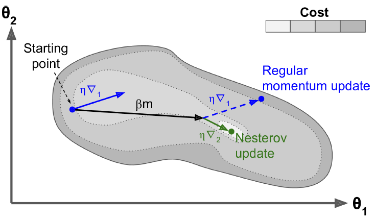
NAG measures the gradient slightly ahead, in the direction of the current momentum, not at the current $θ$ :

m^{(k + 1)} = γ m^{(k)} - α^{(k)} \nabla J (θ^{(k)} + γ m^{(k)}),

θ^{(k + 1)} = θ^{(k)} + m^{(k + 1)} .

The momentum vector usually already points toward the optimum, so the lookahead gradient is a better estimate.

Regular momentum versus Nesterov lookahead

4. AdaGrad

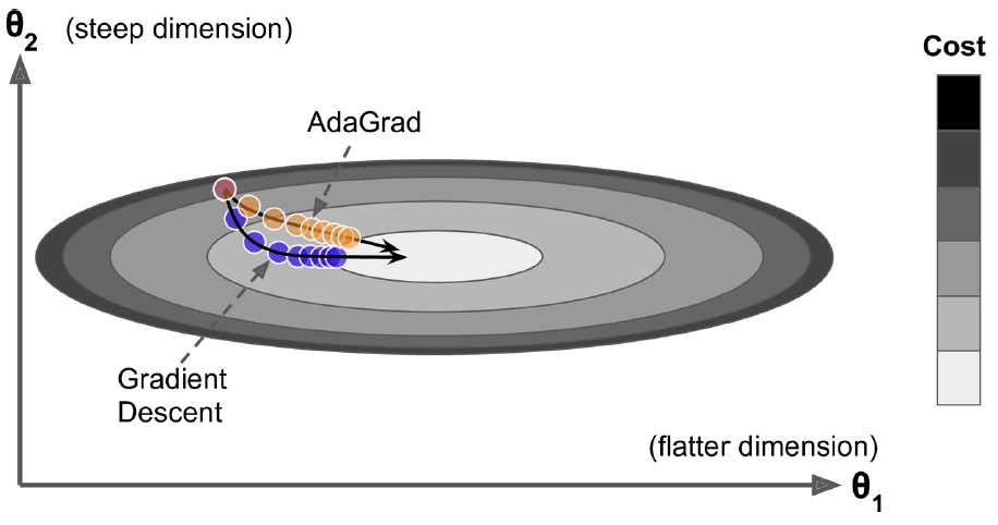
On a long thin valley, gradient descent dives down the steep walls, then creeps along the floor. AdaGrad scales down the gradient on the steep coordinates:

s^{(k + 1)} = s^{(k)} + \nabla J (θ^{(k)}) \otimes \nabla J (θ^{(k)}),

θ^{(k + 1)} = θ^{(k)} - α^{(k)} \nabla J (θ^{(k)}) ⊘ \sqrt{s^{(k + 1)} + ϵ} .

$\otimes$ and $⊘$ are elementwise. $s$ accumulates squared gradients. $ϵ$ (often $10^{- 10}$ ) avoids division by zero.

That is an adaptive learning rate: steep directions decay faster than gentle ones. Updates point more toward the global optimum, and $α$ needs less tuning.

On simple quadratics this works. On deep nets AdaGrad often stops too early: $s$ grows until the effective rate is essentially zero. Do not train a deep net with it. Know it so the later adaptive methods make sense.

AdaGrad correcting the path in a long valley

5. RMSProp

AdaGrad remembers every squared gradient. RMSProp remembers a recent average, with exponential decay:

s^{(k + 1)} = γ s^{(k)} + (1 - γ) \nabla J (θ^{(k)}) \otimes \nabla J (θ^{(k)}),

and the same $θ$ update as AdaGrad. Typical $γ = 0.9$ .

6. Why not Hessians

Everything above uses first derivatives (Jacobians). Second-order methods use Hessians. For $n$ parameters you store on the order of $n^{2}$ Hessian entries per output, versus $n$ Jacobian entries. Deep nets have tens of thousands of parameters. The Hessian often will not fit in memory; computing it is too slow even when it does.

7. Learning-rate schedules

If $α$ is too small, you will get there, late.

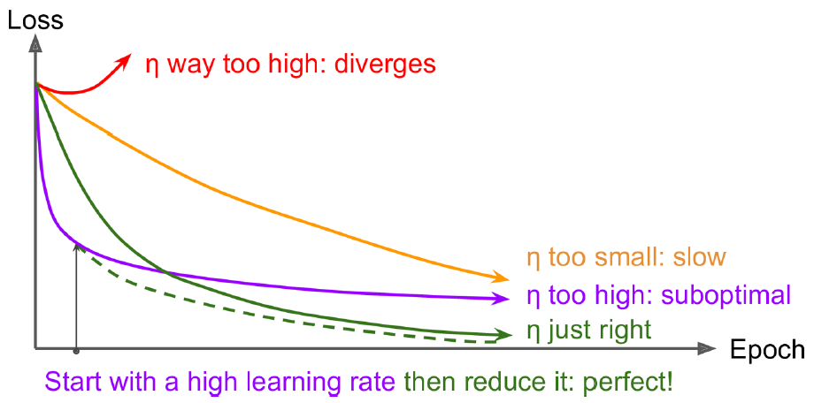
Loss versus iteration for different learning rates

One hunt: start large, divide by 3 until training stops diverging. You land near a rate that learns quickly and still converges.

Other schedules, with iteration $k$ and a scale $s$ :

Schedule	Rule
Power	$α^{(k)} = α^{(0)} / (1 + k / s)^{c}$
Exponential	$α^{(k)} = α^{(0)} {0.1}^{k / s}$
Piecewise constant	e.g. $0.1$ for five epochs, then $0.001$ for fifty, …
Performance	Every $N$ steps, if validation error has stalled, multiply $α$ by $λ$ (same idea as early stopping)

Practice

If momentum uses $γ = 0.9$ , how does terminal velocity compare to a plain gradient step of the same $α$ ?
AdaGrad and RMSProp share an adaptive $s$ . What does RMSProp change so that training need not freeze?
Nesterov evaluates $\nabla J$ where, relative to ordinary momentum?

Ahmad Mousavi