3.1 Constrained Optimization

Lagrange multipliers, the primal, and the dual.

These notes walk through the lecture slides. The original deck is unchanged; use (slides) on the course hub if you want that PDF.

The figures follow Deisenroth, Faisal, and Ong, Mathematics for Machine Learning.

1. Extra conditions on $θ$

Unconstrained: ${min}_{θ} J (θ)$ with $J : ℝ^{l} \to ℝ$ . Constrained: the same min, plus real-valued $g_{i}$ that $θ$ must obey,

{min}_{θ} J (θ) subject to g_{i} (θ) \leq 0, i = 1, \dots, m .

The feasible set can mix equalities and inequalities:

S = {θ : g_{i} (θ) = 0 or g_{i} (θ) \leq 0} .

$J$ and the $g_{i}$ need not be convex. The LP and QP notes take the convex case.

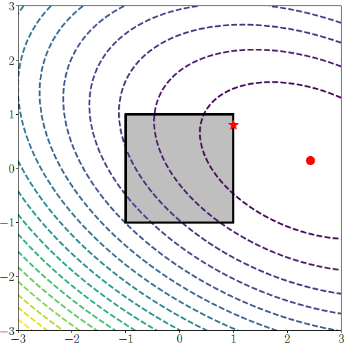
A box $- 1 \leq θ_{j} \leq 1$ is already a constraint set. The unconstrained min can fall outside the box. The constrained min is then on the boundary (the star, not the circle).

Unconstrained min versus a box constraint

2. The primal

The primal is the original problem in $θ$ : minimize $J$ subject to $g_{i} (θ) \leq 0$ . Its solution is the feasible $θ$ you actually want, and the optimal $J$ . Direct search can be ugly once the constraints or $J$ are messy.

Why turn it into an unconstrained problem in more variables?

Reason	What you get
Simplicity	Most solvers are written for unconstrained maps
Algorithms	You can use methods from Week 2
Theory	Stationarity and convergence statements are cleaner
Hard problems	Nonlinear / nonconvex constraints become a Lagrangian you can differentiate

3. The Lagrangian

For inequalities $g_{i} (θ) \leq 0$ ,

ℒ (θ, λ) = J (θ) - \sum_{i = 1}^{m} λ_{i} g_{i} (θ) = J (θ) - λ^{⊤} 𝐠 (θ),

with multipliers $λ \in ℝ^{m}$ . (Sign conventions differ across books; stay consistent with the slide that introduced $g_{i}$ .)

Stationarity of the Lagrangian:

\nabla_{θ} ℒ (θ, λ) = 0, \nabla_{λ} ℒ (θ, λ) = 0 .

A multiplier is the rate of change of $J$ if you nudge the corresponding constraint. It is the price of that constraint.

4. The dual

Minimize $ℒ$ in $θ$ first (when that min is easy). What remains is a function of $λ$ :

D (λ) = {min}_{θ} ℒ (θ; λ) .

The Lagrange dual is

{max}_{λ \in ℝ^{m}} D (λ) subject to λ \geq 0 .

What the dual gives you	Why it matters
A lower bound on the primal min	You can score a candidate $θ$
Multipliers as sensitivities	How much $J$ moves if a constraint moves
Sometimes a cheaper solve	Dual decomposition, cutting planes; $m$ vs $l$ can flip which problem is small

5. SVM as a constrained problem

Soft-margin SVM is already in this shape:

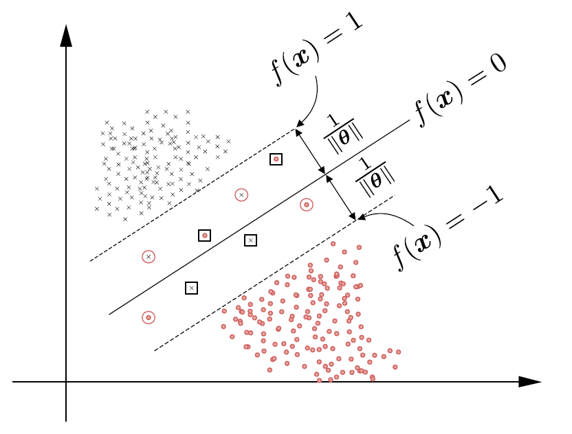
{min}_{θ \in ℝ^{l}} & \frac{1}{2} ‖ θ ‖^{2} + C \sum_{n = 1}^{N} ξ_{n} subject to & y_{n} (x_{n}^{⊤} θ + b) \geq 1 - ξ_{n}, ξ_{n} \geq 0 .

Maximum-margin hyperplane

Form the Lagrangian, pass to the dual, and the multipliers become the story of which points sit on the margin. Notes 3.2 and 3.3 write the same move for an LP and a QP. Week 5 returns to this primal.

6. Practice

What does a Lagrange multiplier charge you for?
In the box-constraint picture, why can the star (constrained min) differ from the circle (unconstrained min)?
Why might you solve the dual instead of the primal, even though the primal is the problem you stated?

Ahmad Mousavi

1. Extra conditions on θ