
10.1 Clustering and K-Means
Partition points into spherical clusters.
These notes walk through the lecture slides. The original deck is unchanged; use (slides) on the course hub if you want that PDF.
Figures and notes follow Géron, Hands-On Machine Learning; Deisenroth, Faisal, and Ong, Mathematics for Machine Learning; and Theodoridis.
1. Central idea
Clustering groups similar instances. No labels.
- Customer segmentation. Split customers by behavior, purchases, or how they interact. Different groups, different products and messages.
- Data analysis. Find the clumps first. Then look at each clump, not at every row at once.
- Dimensionality reduction. Represent a cloud by its clusters instead of by every point. Useful when you want a picture of high-dimensional data.
- Anomaly detection. A point that fits no cluster is a candidate outlier: a defect, a fraud, odd behavior.
- Semi-supervised learning. A few labels, then copy each label onto the rest of its cluster.
- Image segmentation. Cluster pixels by color. Replace each pixel by the mean color of its cluster; fewer colors, easier objects to track.
2. -means
Lloyd proposed it at Bell Labs in 1957 for pulse-code modulation; it left the company in 1982 as “Least square quantization in PCM.” Fast. Often a few iterations.
Write for the index sets of the clusters. They partition the observations:
- — every row sits in some cluster.
- for — clusters do not overlap.
A good clustering makes within-cluster variation small. Solve
Partition so the total within-cluster variation, summed over all clusters, is as small as possible.
A typical is squared Euclidean distance:
where is the number of observations in cluster . All pairwise squared distances inside the cluster, divided by the cluster size.
3. Algorithm
- Initialization. Pick centroids. Random data points, or -means++ (below).
- Assignment. Each point goes to the nearest centroid. Euclidean distance is the usual metric; others are allowed. That step is the partition.
- Update. Each centroid becomes the mean of the points assigned to it.
- Convergence. Stop when centroids (or assignments) barely move.
- Repeat steps 2–4. Each pass tries to cut total within-cluster variation.
4. Why two runs disagree
Random starts. Different initial centroids, different assignments and final centers.
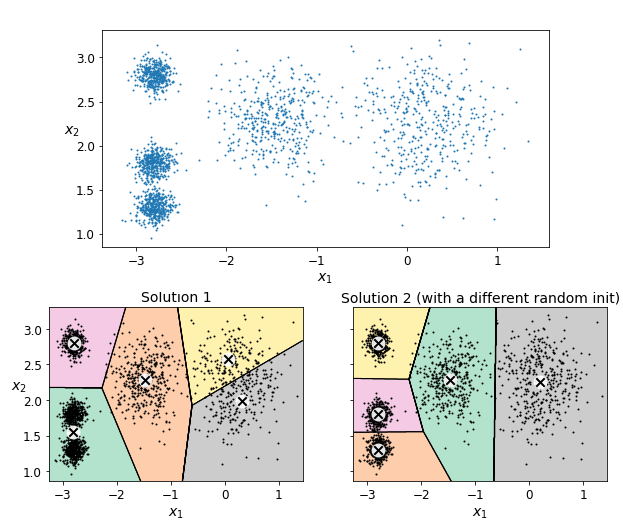
The objective has local optima. A new start can land in a different hole. The stopping rule can also fire on a slightly different iterate.
-means++ (Arthur and Vassilvitskii, 2006) is a better start than uniform draws:
- Draw uniformly from the data.
- Draw the next as instance with probability
where is the distance from to the nearest centroid already chosen. Far points are more likely. - Repeat until you have centroids.
Then ordinary -means. Suboptimal solutions become rarer, so you can cut n_init. In scikit-learn, init="k-means++" is the default.
Elkan. Skip many distance computations with the triangle inequality () and with lower and upper bounds on distances to centroids (Elkan, 2003). Set algorithm="elkan". Dense data only. Sparse data uses the full algorithm.
5. Evaluation
| Tool | What it tells you |
|---|---|
| Inertia | Within-cluster sum of squares. Lower is tighter. |
| Silhouette score | Cohesion inside a cluster versus separation from others. Range to ; higher is better. |
| Elbow method | Plot inertia against . The “elbow” is where the drop flattens — a candidate for . |
| Adjusted Rand index (ARI) | Agreement with another clustering. Range to . |
| Visual inspection | Scatter plots (or similar). Do the clumps look real? |
| Cross-validation | Holdout or -fold, if you have a way to score unseen rows. |
6. Limits
-means is a poor fit when clusters have varying sizes, different densities, or non-spherical shapes.
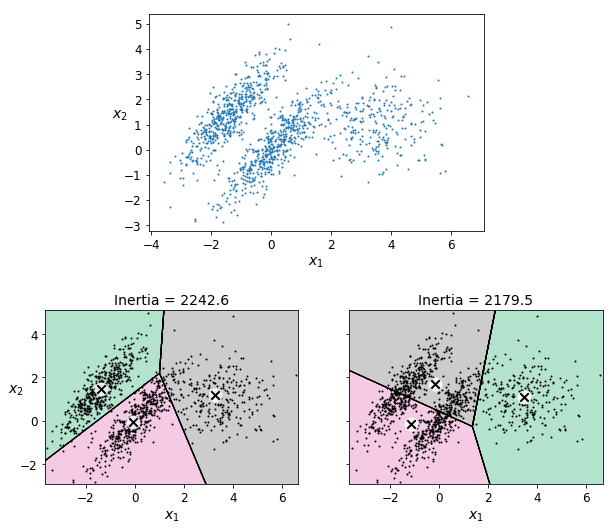
Practice
-
-means assumes spherical clusters. Give a data set where that is wrong.
-
What do you do when is not given?
-
Why can two runs on the same matrix return different partitions?