14.1 Autoencoders

Encode, decode, and reconstruct.

These notes walk through the lecture slides. The original deck is unchanged; use (slides) on the course hub if you want that PDF.

Figures and notes follow Géron, Hands-On Machine Learning; Deisenroth, Faisal, and Ong, Mathematics for Machine Learning; and Theodoridis, Machine Learning: A Bayesian and Optimization Perspective.

1. Representation learning

Autoencoders are neural nets that learn a dense latent representation (a coding) of unlabeled inputs.

The coding is usually much smaller than the input, so the same net is a dimensionality-reduction tool. It is also a feature detector, and it can pre-train a deeper net without labels.

Some autoencoders are generative: train on faces, then draw new faces. The net is trying to copy its input. A small coding, or noise, stops it from copying pixel-for-pixel, so the coding has to be an efficient summary. The identity map, under those constraints, is the goal.

2. Applications

Use	What the coding is doing
Dimensionality reduction	Keep the signal; drop coordinates. Visualization and preprocessing.
Anomaly detection	Normal rows reconstruct well. Odd rows do not (fraud, security).
Feature learning	The coding is a feature vector for a later classifier or regressor.
Denoising	Train on noisy inputs, reconstruct the clean ones.
Generative modeling	VAEs and GANs reuse this encoder–decoder shape to draw new samples.

3. Encoder, decoder, reconstruction

An autoencoder maps $x$ to a short coding, then maps that coding back to something that should look like $x$ . Two pieces: an encoder and a decoder.

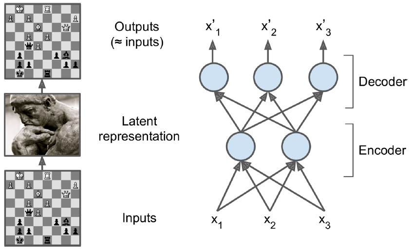
Encoder to a latent coding, decoder back to a reconstruction

The architecture is a multilayer net with one extra rule: the output layer has the same width as the input. The outputs are reconstructions. A reconstruction loss penalizes $\hat{x}$ when it is not $x$ .

4. Loss functions

Which loss you use depends on what $x$ is.

Mean squared error (real-valued reconstructions):

MSE = \frac{1}{N} \sum_{i = 1}^{N} (x_{i} - {\hat{x}}_{i})^{2},

where ${\hat{x}}_{i}$ is the reconstruction.

Binary cross-entropy (binary data):

BCE = - \frac{1}{N} \sum_{i = 1}^{N} (x_{i} \log ({\hat{x}}_{i}) + (1 - x_{i}) \log (1 - {\hat{x}}_{i})) .

Categorical cross-entropy (one-hot rows, $C$ categories):

CCE = - \frac{1}{N} \sum_{i = 1}^{N} \sum_{j = 1}^{C} x_{i j} \log ({\hat{x}}_{i j}) .

5. Linear autoencoders and PCA

A linear autoencoder has no activation functions. It compresses, then reconstructs. That is the same job as PCA: keep a low-dimensional summary that still explains variance.

PCA’s axes are orthogonal principal components. A linear autoencoder does not force orthogonality; with squared loss it still lands close to PCA. Add activations and it can follow nonlinear structure.

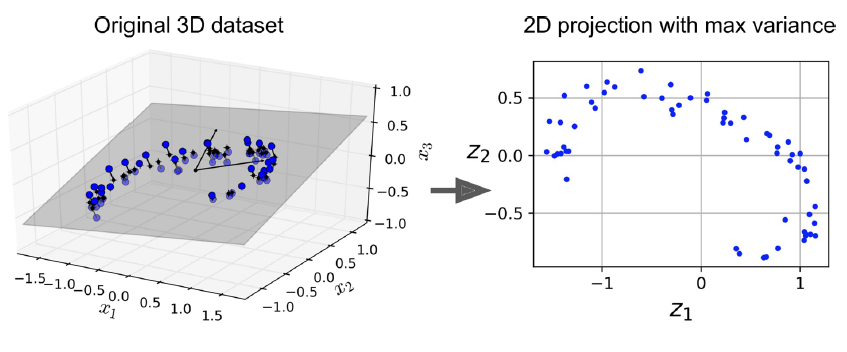
3D data projected to a 2D max-variance plane

The slide sketch is a 3-to-2 encoder and a 2-to-3 decoder, trained with MSE and SGD. Both PCA and this linear net are unsupervised.

6. Stacked autoencoders

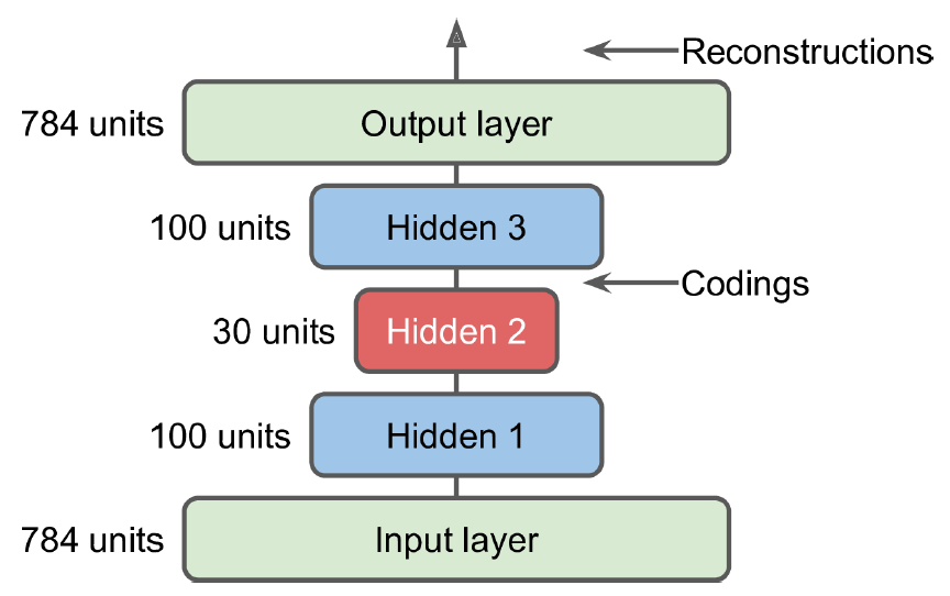
Give the net several hidden layers and it is a stacked autoencoder (a deep autoencoder). Extra layers buy more complex codings.

The usual picture is symmetric about the coding layer: wide, then narrow, then wide again. Deeper layers see more abstract features.

Stacked autoencoder, symmetric about a 30-unit coding

Practice

A linear autoencoder with squared loss is close to which classical method?
Why must the output layer have the same width as the input?
Name two uses of an autoencoder besides dimensionality reduction.

Ahmad Mousavi