11.1 Statistics: Tests

1. Question, then evidence

A test is the last step, not the first. A useful order:

1. a question you can say in words
2. EDA (a plot, a table)
3. a model that matches the question
4. a test saved as an object
5. a sentence a reader can use

Always assign the test. Printing it once is not enough if you later want the p-value or the interval.

library(tidyverse)
library(palmerpenguins)

tt <- t.test(mpg ~ factor(am), data = mtcars)
tt

## 
##  Welch Two Sample t-test
## 
## data:  mpg by factor(am)
## t = -3.7671, df = 18.332, p-value = 0.001374
## alternative hypothesis: true difference in means between group 0 and group 1 is not equal to 0
## 95 percent confidence interval:
##  -11.280194  -3.209684
## sample estimates:
## mean in group 0 mean in group 1 
##        17.14737        24.39231

tt$p.value

## [1] 0.001373638

tt$estimate

## mean in group 0 mean in group 1 
##        17.14737        24.39231

Sleuth3 has the classic two-sample tables from The Statistical Sleuth. Install once in the console, then load a table by name:

install.packages("Sleuth3")
data("case0201", package = "Sleuth3")

case0201 is wide: Cross and Self are two numeric columns. t.test(Cross, Self) is the two-vector form. The formula form needs a long table. If Sleuth3 is not installed, use palmerpenguins or mtcars. Those are the fallbacks for the rest of this note.

2. Two-sample t.test()

Plot first. A boxplot of the numeric variable by the two-level group tells you whether the question is even interesting.

ggplot(mtcars, aes(x = factor(am), y = mpg)) +
  geom_boxplot() +
  theme_bw()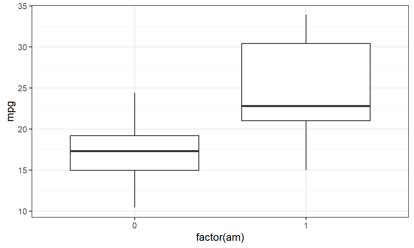

Then the test. The formula is y ~ group. The grouping variable should have exactly two levels.

tt <- t.test(mpg ~ factor(am), data = mtcars)

species in penguins has three levels. Filter to a pair, then droplevels() so the unused level is gone. Without that, t.test() stops.

penguins2 <- penguins |>
  filter(species %in% c("Adelie", "Gentoo")) |>
  droplevels()

ggplot(penguins2, aes(x = species, y = bill_length_mm)) +
  geom_boxplot() +
  theme_bw()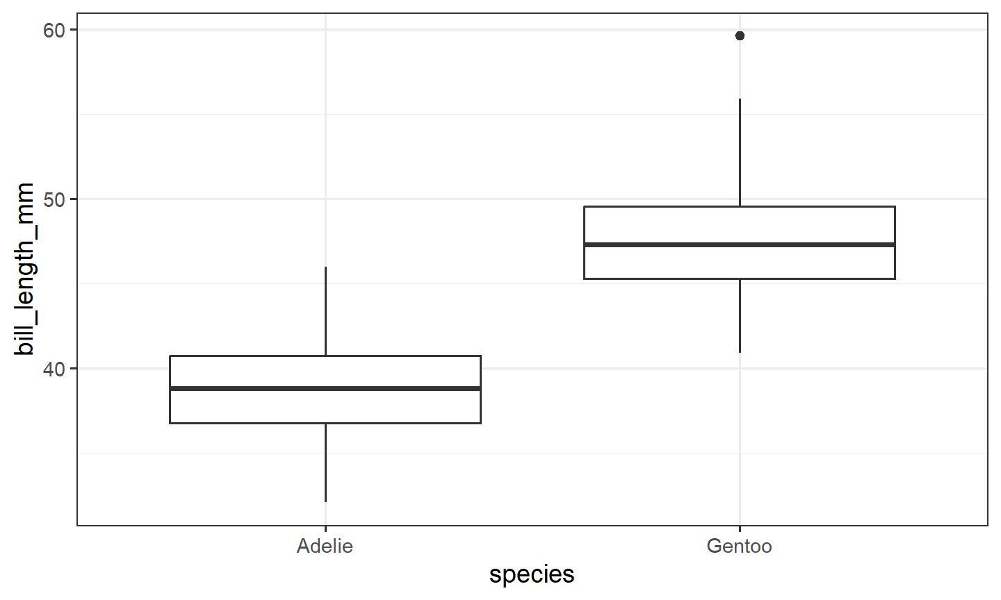

tt_bill <- t.test(bill_length_mm ~ species, data = penguins2)

case0201 after a pivot is the same pattern:

case0201 |>
  pivot_longer(everything(), names_to = "type", values_to = "height") |>
  t.test(height ~ type, data = _)

## Error:
## ! object 'case0201' not found

Default t.test() does not assume equal variances (Welch). That is the usual choice.

3. H0 and the p-value

State H0 in words before you look at the number.

For the penguin pair: mean bill length is the same for Adelie and Gentoo. For mtcars: mean mpg is the same for the two transmission codes.

The p-value is evidence against that H0. A small p-value means the data would be surprising if H0 were true. It is not a stamp that the result is “real,” and 0.05 is not a magic cutoff. Report the p-value, the estimates, and the interval. Then write the sentence.

4. ANOVA and nested models

Three or more groups: aov(y ~ factor), then summary(). Save the object.

fit_aov <- aov(bill_length_mm ~ species, data = penguins)
summary(fit_aov)

##              Df Sum Sq Mean Sq F value Pr(>F)    
## species       2   7194    3597   410.6 <2e-16 ***
## Residuals   339   2970       9                   
## ---
## Signif. codes:  0 '***' 0.001 '**' 0.01 '*' 0.05 '.' 0.1 ' ' 1
## 2 observations deleted due to missingness

H0 in words: mean bill length is the same for Adelie, Chinstrap, and Gentoo. iris (Sepal.Length ~ Species) and mtcars (mpg ~ factor(cyl)) are the no-package backups. Sleuth3 case0501 is Lifetime ~ Treatment if you have the package.

anova() compares nested models. The smaller model is a special case of the larger one.

m1 <- lm(mpg ~ wt, data = mtcars)
m2 <- lm(mpg ~ wt + hp, data = mtcars)
cmp <- anova(m1, m2)
cmp

## Analysis of Variance Table
## 
## Model 1: mpg ~ wt
## Model 2: mpg ~ wt + hp
##   Res.Df    RSS Df Sum of Sq      F   Pr(>F)   
## 1     30 278.32                                
## 2     29 195.05  1    83.274 12.381 0.001451 **
## ---
## Signif. codes:  0 '***' 0.001 '**' 0.01 '*' 0.05 '.' 0.1 ' ' 1

H0: once wt is in the model, hp does not improve the fit. Same rule: save cmp, read the p-value as evidence against that H0, not as a 0.05 switch.

aov() is the one-factor (or multi-factor) fit. anova() is the comparison. Do not mix the two names by accident.

5. Practice

1. Boxplot and two-sample t.test() for a numeric variable by a two-level group. Use mpg ~ factor(am) in mtcars, or Adelie vs Gentoo bill length in penguins (filter, then droplevels()). If you have Sleuth3, do case0201 as well. State H0 in words. Save the test object.
2. aov() of a numeric variable by a factor with three or more levels (bill_length_mm ~ species, or mpg ~ factor(cyl), or Sepal.Length ~ Species). Save the fit. State H0 in words.