11.2 Statistics: Regression and Summaries

1. Fit a linear model

lm(y ~ x1 + x2) is ordinary least squares. Save the fit. The same lifecycle as note 11.1 still applies: question, plot, model, then a sentence.

library(tidyverse)
library(palmerpenguins)

fit <- lm(mpg ~ wt + hp, data = mtcars)

wt is weight; hp is horsepower. Both are in mtcars, which is built in. palmerpenguins is the other table this note uses (bill_length_mm ~ flipper_length_mm + body_mass_g). If Sleuth3 is installed you can load a Sleuth regression table the same way as in 11.1 (install.packages("Sleuth3") once, then data("case0201", package = "Sleuth3") is the two-sample table; pick a later case* with a numeric response for regression). The examples below stay on mtcars and penguins so they run without extra files.

Plot the main relationship before you trust the coefficients:

ggplot(mtcars, aes(x = wt, y = mpg)) +
  geom_point() +
  geom_smooth(method = lm, se = FALSE) +
  theme_bw()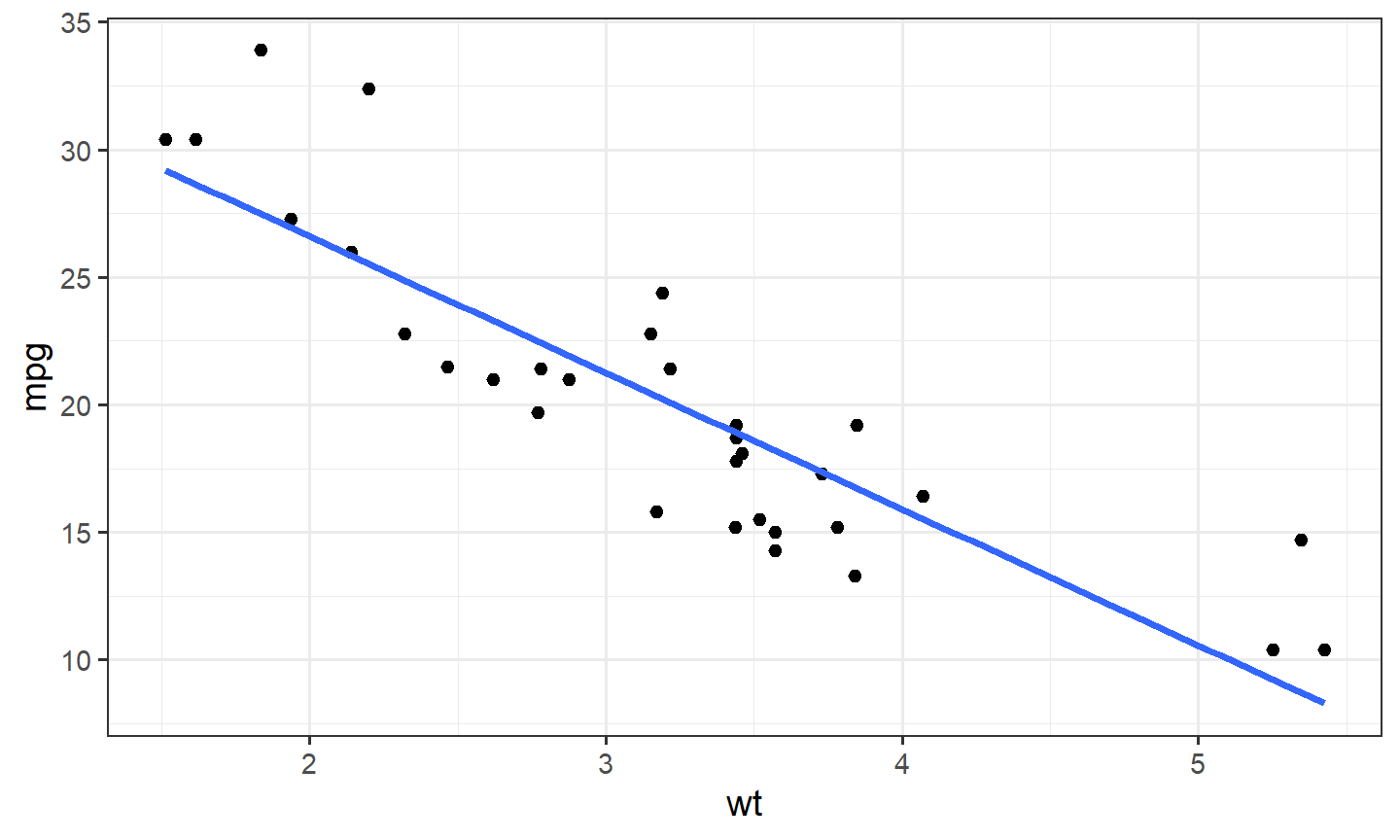

2. Read the fit

Four things you will actually use:

summary(fit)

## 
## Call:
## lm(formula = mpg ~ wt + hp, data = mtcars)
## 
## Residuals:
##    Min     1Q Median     3Q    Max 
## -3.941 -1.600 -0.182  1.050  5.854 
## 
## Coefficients:
##             Estimate Std. Error t value Pr(>|t|)    
## (Intercept) 37.22727    1.59879  23.285  < 2e-16 ***
## wt          -3.87783    0.63273  -6.129 1.12e-06 ***
## hp          -0.03177    0.00903  -3.519  0.00145 ** 
## ---
## Signif. codes:  0 '***' 0.001 '**' 0.01 '*' 0.05 '.' 0.1 ' ' 1
## 
## Residual standard error: 2.593 on 29 degrees of freedom
## Multiple R-squared:  0.8268, Adjusted R-squared:  0.8148 
## F-statistic: 69.21 on 2 and 29 DF,  p-value: 9.109e-12

coef(fit)

## (Intercept)          wt          hp 
## 37.22727012 -3.87783074 -0.03177295

confint(fit)

##                   2.5 %      97.5 %
## (Intercept) 33.95738245 40.49715778
## wt          -5.17191604 -2.58374544
## hp          -0.05024078 -0.01330512

broom::tidy(fit, conf.int = TRUE)

## # A tibble: 3 × 7
##   term        estimate std.error statistic  p.value conf.low conf.high
##   <chr>          <dbl>     <dbl>     <dbl>    <dbl>    <dbl>     <dbl>
## 1 (Intercept)  37.2      1.60        23.3  2.57e-20  34.0      40.5   
## 2 wt           -3.88     0.633       -6.13 1.12e- 6  -5.17     -2.58  
## 3 hp           -0.0318   0.00903     -3.52 1.45e- 3  -0.0502   -0.0133

summary() is the printed report: coefficients, standard errors, t statistics, p-values, and R-squared. coef() is just the estimates. confint() is the interval for each coefficient. broom::tidy() puts the same numbers in a tibble you can pipe.

Install broom once in the console if it is missing. Do not put install.packages() in the Quarto file.

Read one coefficient in words. For mpg ~ wt + hp, the wt number is the change in fitted mpg associated with a one-unit change in wt holding hp fixed. The p-value on that row is evidence against “this coefficient is zero,” not a quality stamp for the whole model.

3. Residual plots

A residual is observed minus fitted. If the model is a good description, residuals look like unstructured noise around zero.

plot(fit, which = 1)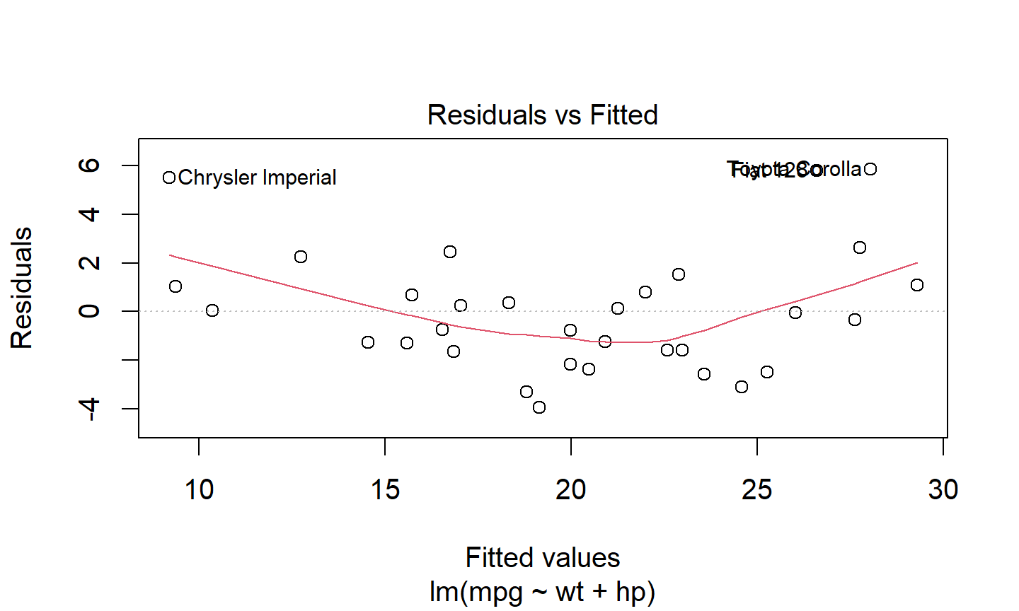

plot(fit, which = 2)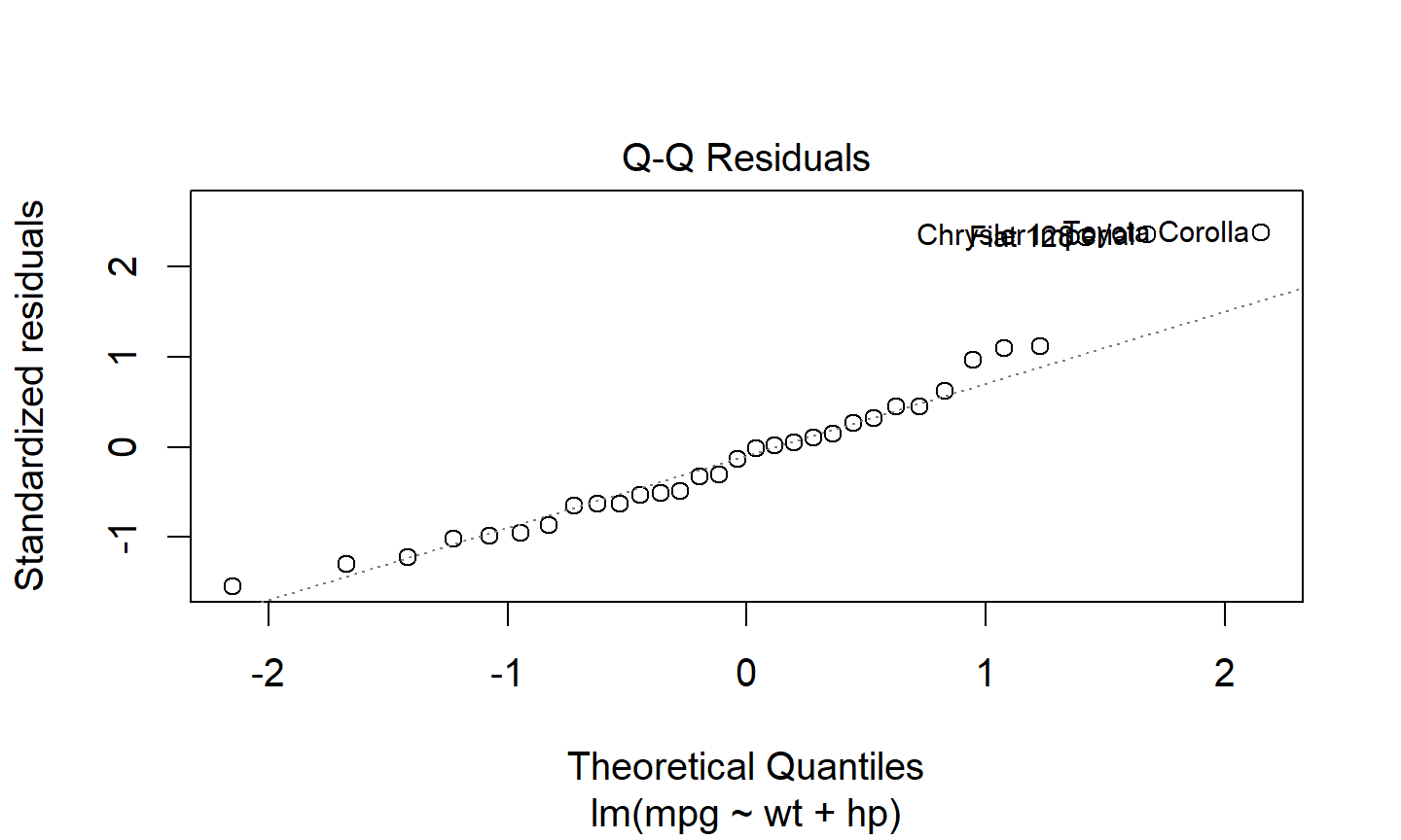

which = 1 is residuals versus fitted. which = 2 is the normal QQ plot. The ggplot version of the first one:

aug <- broom::augment(fit)

ggplot(aug, aes(x = .fitted, y = .resid)) +
  geom_point() +
  geom_hline(yintercept = 0) +
  geom_smooth(se = FALSE) +
  theme_bw()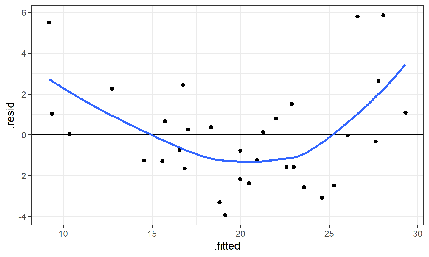

If the residual cloud fans out (small spread on the left, wide on the right), the variance is not constant. A transform of the response is the first thing to try, often log(y):

fit_log <- lm(log(mpg) ~ wt + hp, data = mtcars)
plot(fit_log, which = 1)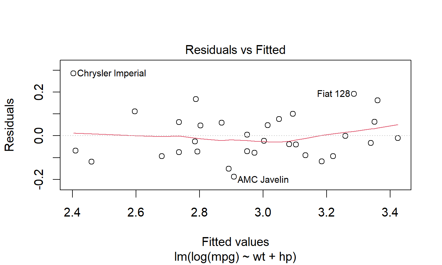

Refit, then look at the residual plot again. Do not transform only because a p-value looked nicer.

4. Numerical summaries

summary() on a data frame is the base-R scan: min, quartiles, mean, max, and a count of NAs for each column.

summary(penguins)

##       species          island    bill_length_mm  bill_depth_mm  
##  Adelie   :152   Biscoe   :168   Min.   :32.10   Min.   :13.10  
##  Chinstrap: 68   Dream    :124   1st Qu.:39.23   1st Qu.:15.60  
##  Gentoo   :124   Torgersen: 52   Median :44.45   Median :17.30  
##                                  Mean   :43.92   Mean   :17.15  
##                                  3rd Qu.:48.50   3rd Qu.:18.70  
##                                  Max.   :59.60   Max.   :21.50  
##                                  NAs    :2       NAs    :2      
##  flipper_length_mm  body_mass_g       sex           year     
##  Min.   :172.0     Min.   :2700   female:165   Min.   :2007  
##  1st Qu.:190.0     1st Qu.:3550   male  :168   1st Qu.:2007  
##  Median :197.0     Median :4050   NAs   : 11   Median :2008  
##  Mean   :200.9     Mean   :4202                Mean   :2008  
##  3rd Qu.:213.0     3rd Qu.:4750                3rd Qu.:2009  
##  Max.   :231.0     Max.   :6300                Max.   :2009  
##  NAs    :2         NAs    :2

summary(mtcars)

##       mpg             cyl             disp             hp       
##  Min.   :10.40   Min.   :4.000   Min.   : 71.1   Min.   : 52.0  
##  1st Qu.:15.43   1st Qu.:4.000   1st Qu.:120.8   1st Qu.: 96.5  
##  Median :19.20   Median :6.000   Median :196.3   Median :123.0  
##  Mean   :20.09   Mean   :6.188   Mean   :230.7   Mean   :146.7  
##  3rd Qu.:22.80   3rd Qu.:8.000   3rd Qu.:326.0   3rd Qu.:180.0  
##  Max.   :33.90   Max.   :8.000   Max.   :472.0   Max.   :335.0  
##       drat             wt             qsec             vs        
##  Min.   :2.760   Min.   :1.513   Min.   :14.50   Min.   :0.0000  
##  1st Qu.:3.080   1st Qu.:2.581   1st Qu.:16.89   1st Qu.:0.0000  
##  Median :3.695   Median :3.325   Median :17.71   Median :0.0000  
##  Mean   :3.597   Mean   :3.217   Mean   :17.85   Mean   :0.4375  
##  3rd Qu.:3.920   3rd Qu.:3.610   3rd Qu.:18.90   3rd Qu.:1.0000  
##  Max.   :4.930   Max.   :5.424   Max.   :22.90   Max.   :1.0000  
##        am              gear            carb      
##  Min.   :0.0000   Min.   :3.000   Min.   :1.000  
##  1st Qu.:0.0000   1st Qu.:3.000   1st Qu.:2.000  
##  Median :0.0000   Median :4.000   Median :2.000  
##  Mean   :0.4062   Mean   :3.688   Mean   :2.812  
##  3rd Qu.:1.0000   3rd Qu.:4.000   3rd Qu.:4.000  
##  Max.   :1.0000   Max.   :5.000   Max.   :8.000

For a tibble of chosen summaries, use across() with a named list. {.col}_{.fn} builds the output names. na.rm belongs on the function, so pass a formula ~ mean(.x, na.rm = TRUE) rather than the bare mean:

penguins |>
  summarize(
    across(
      where(is.numeric),
      list(
        mean = ~ mean(.x, na.rm = TRUE),
        sd = ~ sd(.x, na.rm = TRUE)
      ),
      .names = "{.col}_{.fn}"
    )
  )

## # A tibble: 1 × 10
##   bill_length_mm_mean bill_length_mm_sd bill_depth_mm_mean bill_depth_mm_sd
##                 <dbl>             <dbl>              <dbl>            <dbl>
## 1                43.9              5.46               17.2             1.97
## # ℹ 6 more variables: flipper_length_mm_mean <dbl>, flipper_length_mm_sd <dbl>,
## #   body_mass_g_mean <dbl>, body_mass_g_sd <dbl>, year_mean <dbl>,
## #   year_sd <dbl>

list(mean = mean, sd = sd) is the same idea without na.rm. On penguins that will propagate NAs. Prefer the formula form.

skimr::skim() is a compact one-function scan (types, missingness, mean, sd, quantiles). Install skimr once if you want it. It does not replace a plot.

skimr::skim(penguins)

## Error in `loadNamespace()`:
## ! there is no package called 'skimr'

5. Practice

1. fit <- lm(mpg ~ wt + hp, data = mtcars). Read summary(fit) and confint(fit). Write one sentence that interprets the wt coefficient. Glance at plot(fit, which = 1).
2. across() summaries of every numeric column in penguins or mtcars: mean and sd, .names = "{.col}_{.fn}", na.rm via ~ mean(.x, na.rm = TRUE). If skimr is installed, run skim() on the same table.