4.2 Vision Transformers

DATA 443/643 · Week 4 · PDF · Slides

Non-overlapping patches, a linear map, positions, no causal mask.

These notes match the lecture slides. Use (slides) on the course hub for the deck.

A vision transformer (ViT) is the Week 3 block on patches instead of words. Once an image is a sequence, every later trick in this course (attention, positions, [CLS], CLIP’s image tower) applies. The recipe is patchify, linear map, positions, no causal mask. You do not train a ViT from random pixels in this hour; you learn to count tokens and reuse the stack.

1. What a vision transformer (ViT) is

A ViT treats an image as a sequence of patches. Split a $H\times W$ image into non-overlapping $P\times P$ patches, flatten each patch, and map it with a linear layer to width $d$. Add a learned [CLS] if you classify from one vector, and add positions (a 1-D index, or row–column). Then run a transformer without a causal mask: every patch may look at every patch. Attention without positions is a bag of tiles.

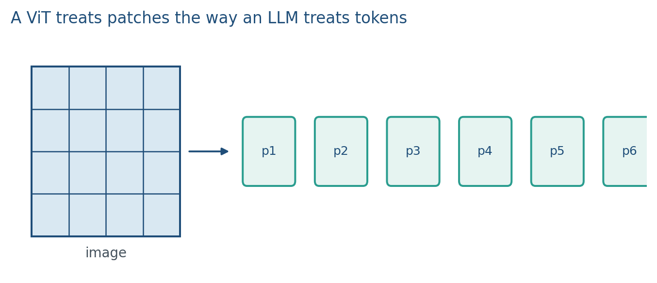
The sequence length for a tiled image is

A CNN shares a small kernel and builds a hierarchy. A ViT sees global context in layer 1, at $O(N^2)$ cost. For a 224 image and $P=16$, $N=196$, which is a short paragraph.

Flattening a $16\times 16\times 3$ patch is $768$ numbers. That linear map is the same as a convolution with kernel $P$, stride $P$, and $d$ output channels. RGB is just three extra channels in the flatten.

Do not count overlapping CNN windows and then write $N=HW/P^2$. ViT patches tile.

2. Why we use it

CNNs were the older default for images. ViT shows that the same block you already use for language can mix patches globally from layer 1. That matters for this course because CLIP’s image tower is often a ViT, and every later “freeze the vision encoder” sentence is freeze patch embed plus transformer.

Scale is the other reason. Dosovitskiy et al. (2021) found that ViTs need more data than ResNets if trained from scratch, and they shine when the image set is large. In this course you will almost always start from a pretrained ViT (CLIP’s image tower, or a Hugging Face checkpoint), not from random pixels. A tiny medical set is the wrong place to train a ViT from scratch.

A smaller patch gives more tokens and a heavier $N^2$ map. Patch size is a method knob, not a default you ignore.

3. Architecture

The boxes are the Week 3 encoder, with a patch embedding instead of a token embedding.

1. Cut the image into non-overlapping patches and flatten each one.
2. Map with a linear layer $E\in {ℝ}^{P_{\mathrm{f}\mathrm{l}\mathrm{a}\mathrm{t}}\times d}$ (for RGB, $P_{\mathrm{f}\mathrm{l}\mathrm{a}\mathrm{t}}=P·P·3$).
3. Optionally prepend a learned [CLS] token.
4. Add positional embeddings. Without them, top and bottom are the same bag.
5. Run encoder blocks: LayerNorm, multi-head self-attention, MLP, residuals. No causal mask.
6. Classify from [CLS] or from a mean-pool of the patch tokens, then a linear head.

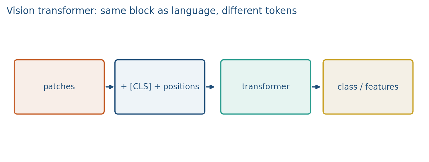
Unlike GPT, a classifier ViT is bidirectional. There is no future patch to hide. Hybrid models put a small CNN stem first, then a transformer on a coarser grid. Same $N$ idea, fewer tokens.

When you later freeze “the vision encoder,” you are freezing patch embed + transformer. You are not freezing a ResNet unless the checkpoint says so.

4. How it works, step by step

Lab 4 flattens patches in numpy. No convolution is required for the cartoon. Do one flatten on the board before the lab.

1. Count patches. Image $H=W=4$, $P=2$, one channel $\Rightarrow$ $N=4$. Standard ImageNet: $224\times 224$, $P=16$, $N=196$. Plus [CLS]: 197 tokens.
2. Flatten one tile. Top-left $2\times 2$ patch $\left[\begin{array}{cc}1& 2\\ 3& 4\end{array}\right]$ becomes $\left[\begin{array}{cccc}1& 2& 3& 4\end{array}\right]$.
3. Linear map. A matrix $W\in {ℝ}^{2\times 4}$ with first row all $0.25$ sends that tile to a 2-D token whose first coordinate is the mean $2.5$.
4. Add positions and [CLS]. The transformer now sees a sequence, not a bag.
5. Attend without a causal mask. Every patch may look at every patch. One attention map with [CLS] has ${197}^2=38809$ scores per head.
6. Pool and classify, or pass the sequence into CLIP as the image tower.

You do not implement ViT from random init in this course. You count patches, you add positions, you reuse Week 3.

A smaller patch ($P=8$ on 224) gives $N=784$ tokens and a heavier $N^2$ map. That is why 16 is the default: enough spatial pieces, still a short sequence.

5. Mathematical formulas

For patch size $p\times p$ and image $H\times W$, the tiled sequence length is

when both axes divide. With a [CLS] token the transformer sees $T+1$ positions.

Let $P$ be the matrix of flattened patches (one row per tile). A linear patch embedding and positions give

then the usual encoder stack. The patch map $W_e$ is equivalent to a convolution with kernel size $p$, stride $p$, and $d$ output channels.

Attention cost is quadratic in the number of tokens: $O((T+1{)}^2)$ scores per head if you include [CLS].

6. Positive points and negative points

Positive.

• Global mixing from layer 1, with the same encoder code as language.
• A pretrained ViT (CLIP’s image tower, a Hugging Face checkpoint) is the default backbone later in the course.
• Patch size lets you trade spatial detail against sequence length.

Negative.

• Attention is quadratic in the number of patches.
• From-scratch ViTs want large image sets or a strong recipe; small medical sets prefer a pretrained tower or a CNN.
• Forgetting positions makes top and bottom indistinguishable.
• A GPT causal mask on patches hides a “future” that does not exist.

When not to. Do not train a ViT from scratch on 800 scans. Start from a pretrained tower. Do not count overlapping CNN windows and then write $N=HW/P^2$.

7. Teaching this note

~16 minutes. Count patches on a square image, flatten one toy $2\times 2$ patch, add [CLS]+positions, then “same block as Week 3, no causal mask.” Play the patch embedding stretch of the Umar Jamil video. Lab 4 will flatten patches in numpy; do one flatten on the board first. Do not train a ViT in this block.

8. Worked example

Image $H=W=4$, $P=2$, 1 channel. Then $N=4$ patches. Top-left patch

flattens to $\left[\begin{array}{cccc}1& 2& 3& 4\end{array}\right]$. A linear map $W\in {ℝ}^{2\times 4}$ with first row all $0.25$ sends it to a 2-D token whose first coordinate is the mean $2.5$.

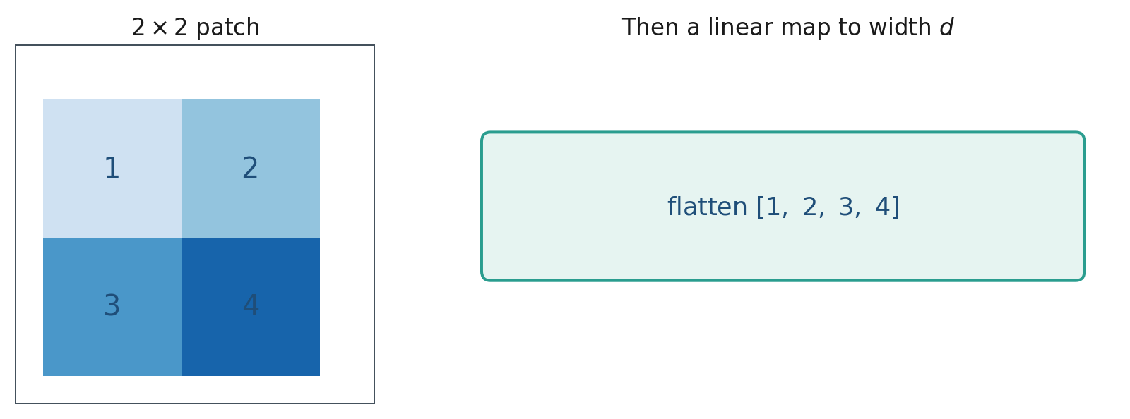
Standard ImageNet: $224\times 224$, $P=16$, $N=196$. Plus [CLS]: 197 tokens. Attention map ${197}^2=38809$ scores per head.

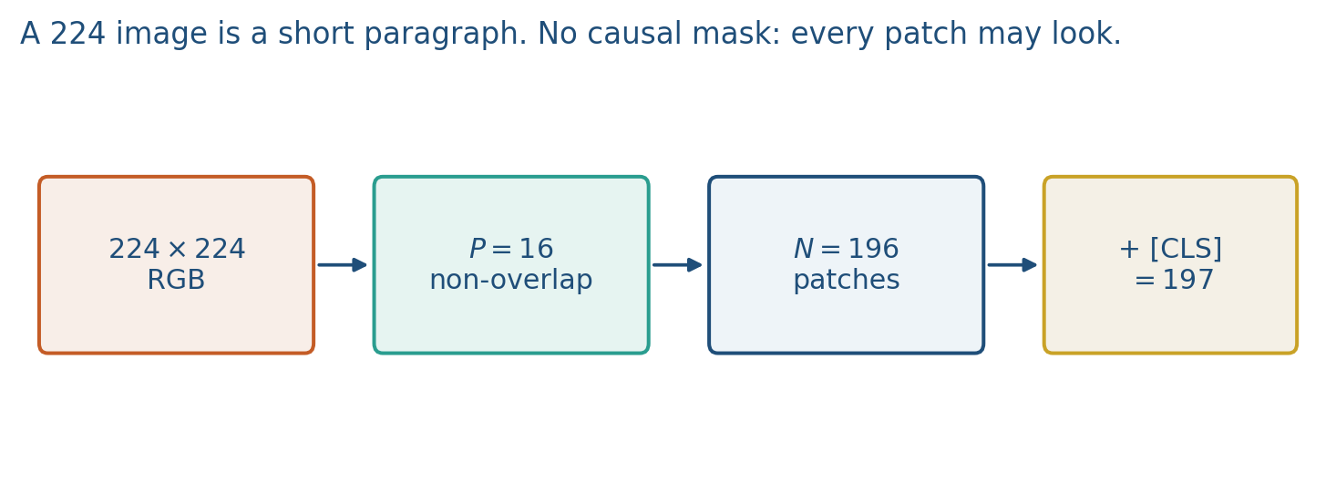
A smaller patch ($P=8$ on 224) gives $N=784$ tokens and a heavier $N^2$ map. That is why 16 is the default: enough spatial pieces, still a short sequence.

You do not implement ViT from random init in this course. You count patches, you add positions, you reuse Week 3.

9. Where students get stuck

• Using overlapping CNN-style windows and then miscounting $N=HW/P^2$.
• Forgetting positions so the model cannot tell top from bottom.
• Putting a GPT causal mask on patches (there is no “next patch” to hide).
• Training a ViT from scratch on a tiny medical set.

10. Video

Watch Umar Jamil: Vision Transformer / VLM walkthrough.

Pause on image patches as tokens, the linear patch embedding, and positional encodings. That is the ViT; CLIP/BLIP wrap extra towers around it.

11. Practice

1. Count tokens for a $384\times 384$ image, patch $16$.

2. Why add positions if attention already sees all patches?

3. A medical image dataset with 800 scans: from-scratch ViT or a pretrained tower? Why?

4. For $224\times 224$, $P=16$, include a [CLS] token. How many tokens enter the transformer? How many scores in one attention map?

5. A $32\times 32$ RGB image, $P=8$. Flatten one patch: how many numbers before the linear map? How many patches in the whole image?

6. Why does a classifier ViT not use a causal mask?

7. The patch linear map is a convolution with which kernel size and stride?