2.2 Vanishing and Exploding Gradients

DATA 443/643 · Week 2 · PDF · Slides

BPTT sums copies of the shared matrix. If the largest |eigenvalue| is below 1, early tokens stop training.

These notes match the lecture slides. Use (slides) on the course hub for the deck.

Backprop through an unrolled RNN multiplies one Jacobian per time step. If those matrices shrink, the early-token gradient vanishes; if they grow, it explodes—either way, long-range learning dies. By the end you should be able to write the product of Jacobians, compare ${0.5}^T$ with ${1.5}^T$, and say why clipping does not restore a vanished signal.

1. What vanishing and exploding gradients are

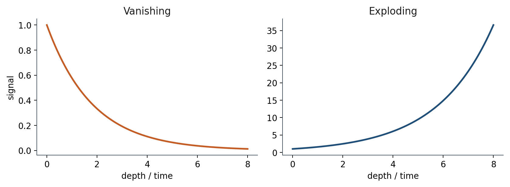
Vanishing (and exploding) gradients are why vanilla RNNs forget. The loss at each step depends on the shared $W_h$. Backprop through the unrolled chain multiplies the same Jacobian many times. If those factors shrink, the gradient on an early token dies. If they grow, activations and gradients explode into NaNs.

The multivariable chain rule says: the gradient with respect to a repeated weight is the sum of the gradient at each copy. That algorithm is backpropagation through time (Werbos 1988).

Wh" src="files/graphics/2.2-vanishing-gradients/bptt.png" />

In practice people often truncate after a few tens of steps so a batch fits in memory. Truncation is an efficiency choice. It does not fix vanishing: a truncated window never sees the token that sat 200 steps back. You do not implement truncated BPTT by hand this week. loss.backward() on nn.RNN is BPTT over the sequence you fed it.

Same product, opposite problem: vanishing is a dead arrow; exploding is a huge one. They are different bugs.

2. Why we use it

You asked the RNN to carry a bit across $T$ steps. The gradient is the only teacher for those early weights. A vanilla RNN can learn “the next word looks like the last few.” It struggles with “the negation was at the start of the review.”

A long-range example, shortened: she tried to print her tickets, left, bought toner, came back, and finally printed her _. The model has to bind the last word to tickets many steps earlier. If the gradient from that last NLL never reaches the early embedding, the net never learns the dependency, and at test time it cannot use it.

Lab 2 is a copy task: the first bit must survive many steps. Vanilla RNNs fail as the gap grows; that is this product, not a PyTorch bug.

This is not only an RNN problem. Any deep stack of Jacobians can vanish or explode. Recurrence is just the case where you multiply by the same $W_h$ over and over (Bengio et al. 1994; Pascanu et al. 2013). Transformers side-step the chain: every token attends to every other token in one step (Week 3). Gates (Week 2.3) were the fix inside the recurrent family.

3. Architecture

Unroll the RNN: $T$ copies of $W_h$. The gradient of $L$ with respect to ${\mathit{h}}_1$ goes through $T-1$ multiplies. There is no extra layer. The architecture is the unrolled chain from note 2.1, now read as a computational graph for BPTT.

The loss at the last token, $L({\mathit{h}}_T)$, depends on ${\mathit{h}}_1$ through

Each factor $\partial {\mathit{h}}_t/\partial {\mathit{h}}_{t-1}$ contains $W_h$ and ${\tanh }^{\prime }$. For $\tanh$, $\left|{\tanh }^{\prime }\right|\le 1$, and it is $\ll 1$ unless the pre-activation sits near 0. Multiplying by the activation Jacobian is almost always a shrink. A product of twenty numbers smaller than 1 is tiny.

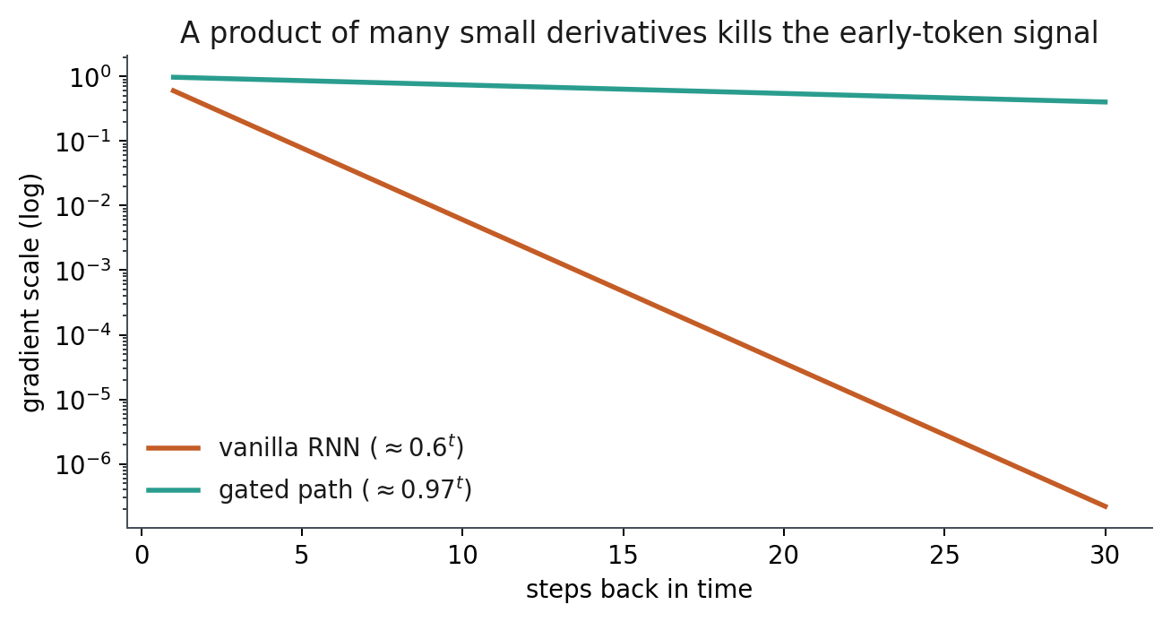
The gated curve is the slogan for LSTM/GRU: keep a path whose multiplier can stay near 1.

4. How it works, step by step

Diagnose with gradient norms versus $T$. In a project, if you still train an RNN on long documents, watch the gradient norm and (if you can) the contribution from early positions. If it is always $\approx 0$ on the start of the sequence, the net is not using the beginning.

Ignore the nonlinearity for a minute. A linear recurrence ${\mathit{h}}_t=W_h{\mathit{h}}_{t-1}$ scales, for large $t$, like $|{\lambda }_{max}{|}^t$, where ${\lambda }_{max}$ is the largest-magnitude eigenvalue of $W_h$. The same fact is often stated with the largest singular value.

• $\left|{\lambda }_{max}\right|<1$: the forward state and the backward signal vanish.
• $\left|{\lambda }_{max}\right|>1$: they explode.
• Exactly 1 in every direction is the unitary dream. Vanilla RNNs do not learn that matrix.

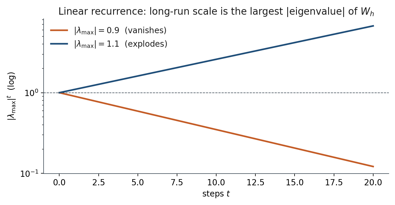
In 1-D, if each factor is $0.5$, ten steps give ${0.5}^{10}\approx 0.001$. The early token still sits in the forward state as a faint trace, but the learning signal is gone.

ReLU is not a rescue: if the pre-activation is negative the unit dies; if $W_h$ is large it blows up. Tanh is the least-bad vanilla default. It is still short memory.

If $\Vert W_h\Vert$ is large, the signal blows up, weights become NaNs, and training stops. Gradient clipping (Pascanu et al. 2013): if $\Vert \mathit{g}\Vert >c$, replace $\mathit{g}$ by $c\mathit{g}/\Vert \mathit{g}\Vert$. Same direction, shorter step.

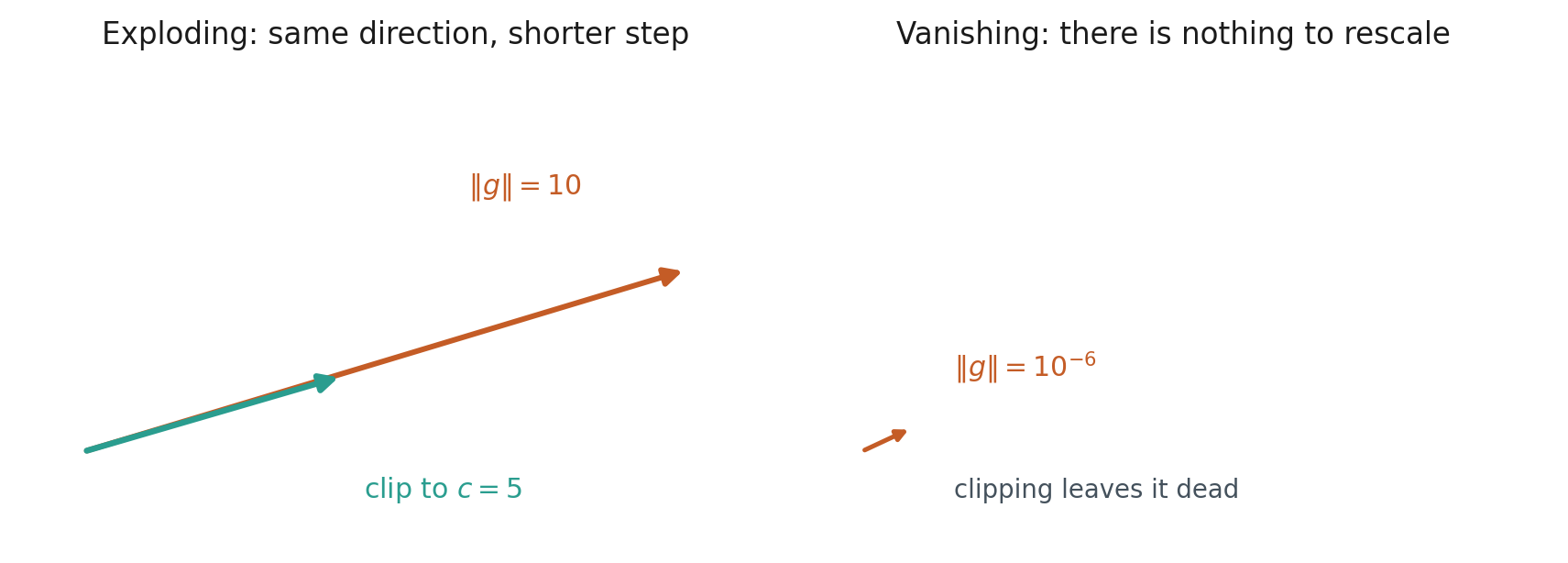
Clipping is the bandage for exploding. It does not fix vanishing. A vanished vector is already near $\mathbf{0}$; multiplying it by 1 does nothing useful. Mitigate exploding with clipping; mitigate vanishing with gates (next note), not by “more layers” of the same cell.

5. Mathematical formulas

The product along the unrolled chain:

Each factor involves $W_h$ and the activation Jacobian. For a $\tanh$ cell, $\partial h_t/\partial h_1$ involves ${\prod }_{s=2}^t{W}_h^{\top }{D}_s$, where $D_s=diag({\tanh }^{\prime }(z_s))$ and $\left|{\tanh }^{\prime }\right|\le 1$.

Linear picture: ${\mathit{h}}_t=W_h{\mathit{h}}_{t-1}$ scales like $|{\lambda }_{max}{|}^t$.

Gradient clipping: if $\Vert \mathit{g}\Vert >c$,

That is the same as $g\leftarrow g·min(1,C/\Vert g\Vert )$ in one dimension. Direction preserved; length capped at $c$.

6. Positive points and negative points

Positive.

• Clipping is cheap: one norm, one possible rescale, and exploding steps stop becoming NaNs.
• The diagnosis is plottable: gradient norms versus $T$, and (in Lab 2) the contribution from early positions.
• Naming vanishing versus exploding as different bugs keeps you from applying the explode bandage to a vanish wound.
• The same product explains why Week 3’s path length of 1 is a big deal.

Negative.

• Clipping does not fix vanishing. A near-zero vector stays near zero.
• Truncated BPTT saves memory; it does not save a dependency that sits outside the window.
• ${\tanh }^{\prime }\le 1$ means the activation Jacobian is almost always a shrink, even before $W_h$ is small.
• ReLU is not a rescue: dead units or explosions, depending on the pre-activation and $\Vert W_h\Vert$.
• Summing gradients over time copies of $W_h$ does not, by itself, save an early token whose Jacobian product is ${10}^{-7}$.

When not to. If the sequence is short enough that the product stays healthy, a vanilla RNN can learn local patterns. Lab 2’s growing gap is the case where you should not keep stacking the same cell and hoping.

7. Teaching this note

~18 minutes. BPTT as a sum over copies, then the product of Jacobians, then the 1-D geometric example (${0.5}^T$ vs ${1.5}^T$), then $|{\lambda }_{max}{|}^t$, then clipping as a cap on a tall arrow. Play the vanishing/exploding segment of the assigned video (about 45:00–58:00; if chapter marks differ, jump to the Jacobian-product board). LSTM details wait for 2.3.

8. Worked example

Scalar RNN: $h_t=\tanh (w{h}_{t-1})$. Then $h_t^{\prime }(h_{t-1})={\tanh }^{\prime }(z_t)w$ with $\left|{\tanh }^{\prime }\right|\le 1$.

Take $w=0.5$ and pretend ${\tanh }^{\prime }=1$ (best case). The factor per step is $0.5$:

Now $w=2$: $2^{10}=1024$. Same chain, opposite disaster.

Linear picture: ${0.9}^{20}\approx 0.12$, ${1.1}^{20}\approx 6.7$. Twenty steps already separate “almost gone” from “several times larger.”

Clipping: gradient $g=50$, threshold $c=5$. New gradient $5$. If instead $g={10}^{-6}$, clipping leaves it at ${10}^{-6}$.

Vector clip: $\mathit{g}=[-6,8]$ has Euclidean norm $10$. With $c=1$, the clipped vector is $\mathit{g}/10=[-0.6,0.8]$.

9. Where students get stuck

• Thinking clipping “fixes RNNs,” including vanishing.
• Forgetting ${\tanh }^{\prime }\le 1$ and blaming only $W_h$.
• Treating truncated BPTT as a vanishing-gradient solution.
• Plotting loss and missing a per-position gradient plot in Lab 2.

10. Video

Watch RNNs and vanishing gradients.

Play the vanishing and exploding segment (roughly 45:00–58:00). Pause on the product of Jacobians and on the plot of gradient size vs. steps back in time. Skip n-gram language modeling and skip NMT.

11. Practice

1. Why is ${\tanh }^{\prime }$ a problem when the state saturates at $\pm 1$?

2. Clipping stops explosions. Why does it not restore a vanished signal?

3. In one sentence: what would you plot in TensorBoard to see this failure in Lab 2?

4. If each Jacobian factor has operator norm $0.8$, the bound on $\Vert \partial h_{20}/\partial h_1\Vert$ is ${0.8}^{19}$. Compute ${0.8}^{10}$ and ${0.8}^{19}$ (calculator is fine). Is the 19-step bound closer to $0.1$ or to $0.01$?

5. A clip threshold $c=1$ meets a gradient of $[-6,8]$ (Euclidean norm $10$). Write the clipped vector.

6. A linear RNN has $|{\lambda }_{max}(W_h)|=0.9$. After 30 steps, is $|{\lambda }_{max}{|}^{30}$ closer to $0.04$ or to $0.4$?

7. Why does summing gradients over time copies of $W_h$ not, by itself, save an early token whose Jacobian product is ${10}^{-7}$?