3.3 The Transformer Block

DATA 443/643 · Week 3 · PDF · Slides

Positions, residual highways, a token-wise MLP, encoder versus decoder.

These notes match the lecture slides. Use (slides) on the course hub for the deck.

A transformer block is attention, a residual add, layer norm, then a token-wise MLP, another residual and norm. Stack $N$ of those. Attention mixes across positions; the MLP mixes across channels at one position. That is the assembly order. By the end you should be able to walk the block, count $4d^2$ versus $8d^2$, and say what GPT drops from a Vaswani decoder.

1. What a transformer block is

A transformer block is attention plus an MLP, with residuals. One layer: (masked) self-attention, residual + LayerNorm, token-wise MLP, residual + LayerNorm. Positions are added on the embeddings before the first block.

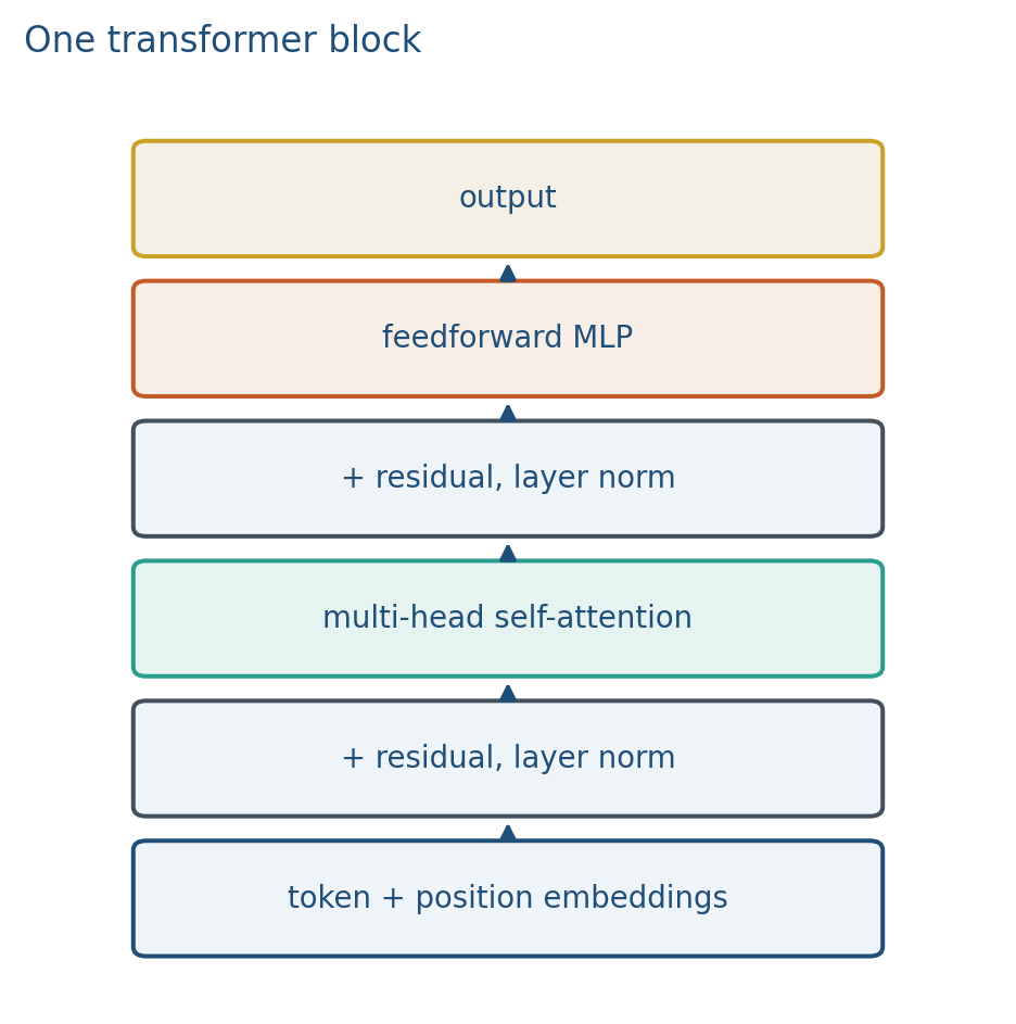
Attention mixes across positions. The MLP mixes channels at one position. Residuals keep a highway so depth trains. Stack $N$ copies of this block; GPT-2 small is $N=12$, $d=768$.

The original transformer has an encoder (bidirectional self-attention on the source) and a decoder (causal self-attention plus cross-attention into the encoder). GPT keeps only a decoder. BERT keeps only an encoder. The block is the same idea; the mask and the extra cross-attention sublayer are the fork (note 3.4).

2. Why we use it

Attention is a set operation: permute the tokens, the weights permute with them. Language is ordered. Without positions, dog bites man and man bites dog can produce the same bag of contextual vectors up to permutation. That is fatal for language.

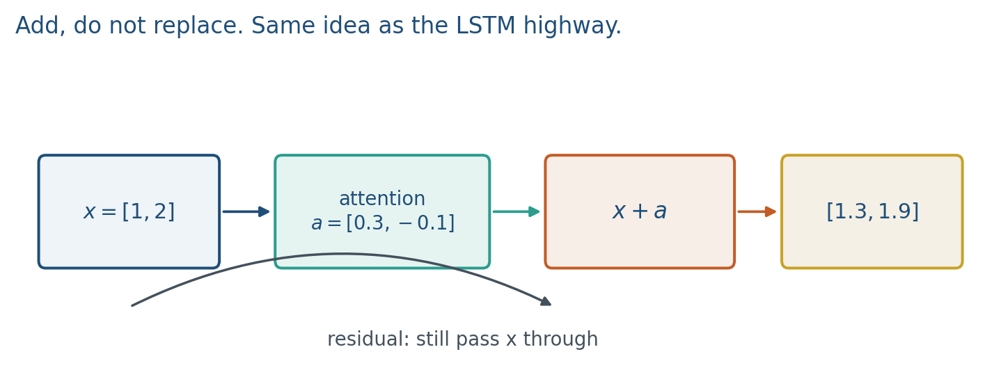
Residuals are another highway, like the LSTM cell, so gradients can skip a messy attention map. Depth is usable because $x\leftarrow x+\mathrm{s}\mathrm{u}\mathrm{b}\mathrm{l}\mathrm{a}\mathrm{y}\mathrm{e}\mathrm{r}(x)$ still passes $x$ through if the sublayer is near zero.

Most of the parameters live in the MLP, not in attention. You stack this block because one mix-across-positions plus one mix-across-channels, repeated, is the default computer of the rest of the course.

3. Architecture

Positional encodings (sinusoids in the original paper, or learned vectors) are added to token embeddings before the first block:

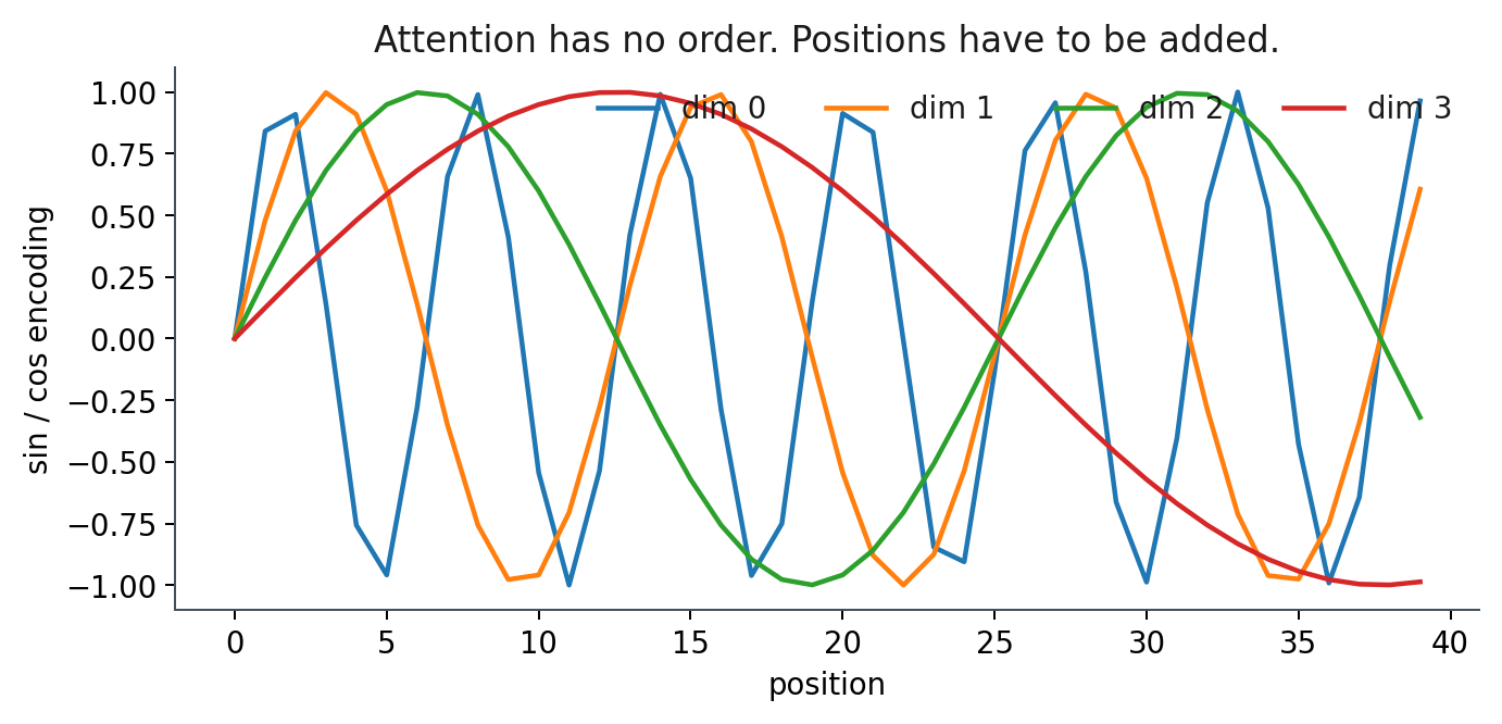
Relative or rotary positions (RoPE) appear in later LLMs. The idea is the same: put order into the vectors because the mixing layer will not. We do not derive RoPE this week.

Residual: add the input of the sublayer to its output.

Layer norm: normalize across features of one token. Pre-norm (layer-norm, then sublayer, then residual) is the usual modern default; it trains more stably at depth. Post-norm (sublayer, residual, then norm) is the 2017 paper. You will see pre_norm in Hugging Face configs. Do not swap them casually and call it an ablation of “the architecture.”

MLP: usually two linear maps with a GELU, hidden width $4d$. Count, roughly: attention’s $W_Q,W_K,W_V,W_O$ are four $d\times d$ maps $\approx 4d^2$. MLP is $d\times 4d$ and $4d\times d$ $\approx 8d^2$. The MLP is heavier.

Decoder-only (GPT): causal mask, no cross-attention. Encoder (BERT): bidirectional self-attention. Encoder–decoder: extra cross-attention. Translation is the original picture.

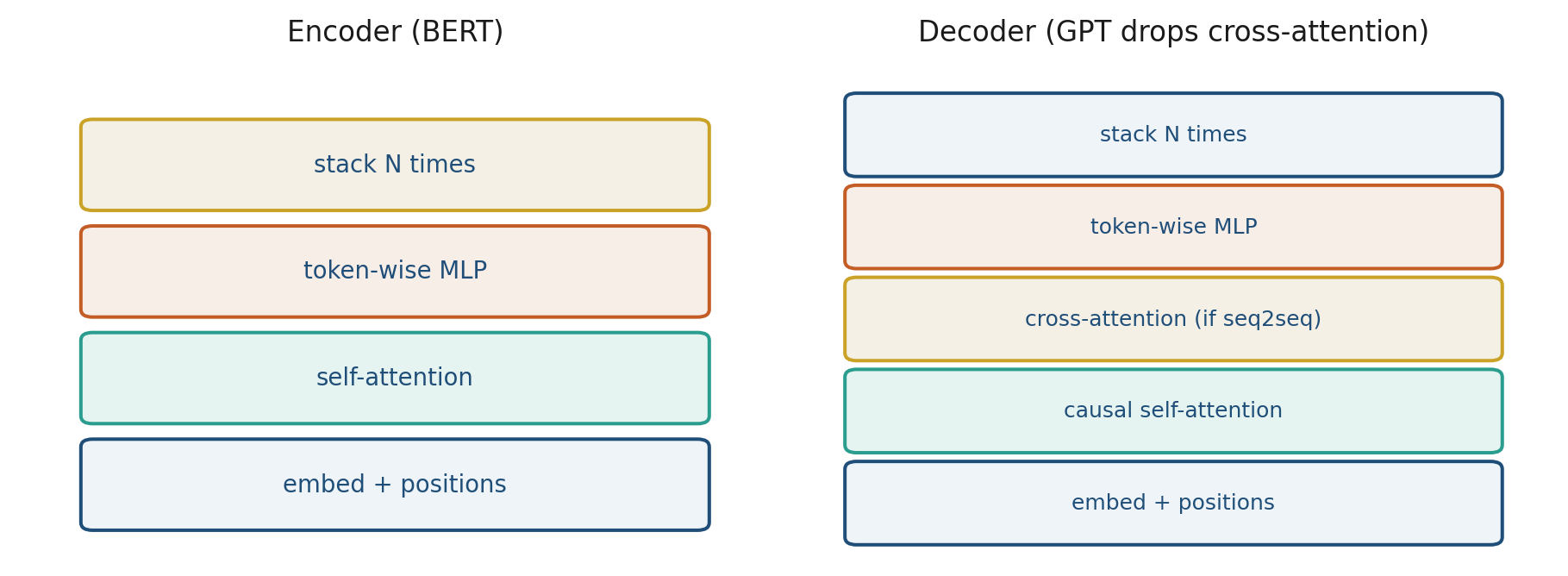
GPT keeps only a decoder (and drops cross-attention: there is no separate encoder). BERT keeps only an encoder. T5 and BART keep both; you do not need both unless the task is sequence-to-sequence.

Cross-attention: queries from the decoder, keys/values from the encoder. Captioning (BLIP, Week 5) uses that pattern with image tokens as the encoder side.

A cartoon of the residual stack (norms omitted) is

Draw residual around sublayers. Pre-norm versus post-norm is a stability knob, not a different model family.

4. How it works, step by step

1. Add a positional vector to each token embedding. Swapping tokens now swaps different vectors, not identical ones.
2. Run (masked) self-attention on the sequence. Mix across positions.
3. Add the residual and apply layer norm (order depends on pre-norm vs post-norm).
4. Run the token-wise MLP (width $4d$, GELU). Mix channels at one position. Residual and norm again.
5. Repeat for $N$ blocks. The next note chooses the mask and the training objective.

If attention were zero (uniform mix that cancels, or a dead head), you still pass $\mathit{x}$ through. That is the highway.

Layer-norm of a two-dimensional vector $\mathit{u}=\left[\begin{array}{c}3\\ 1\end{array}\right]$: mean $2$, population std $1$, so $(1,-1)$. That is per token, across channels, not across the batch.

5. Mathematical formulas

Input to the first block:

Residual around a sublayer:

Cartoon recurrence (norms omitted):

Parameter sketch, ignoring biases: attention $\approx 4d^2$, MLP $\approx 8d^2$. For $d=4$, that is 64 versus 128. For $d=8$, 256 versus 512. The MLP has twice as many.

Layer-norm on one token: subtract the mean of its $d$ channels and divide by their (population) standard deviation, then scale and shift with learned gain and bias. The 2-D drill in the worked example omits $\epsilon$ and the affine parameters.

6. Positive points and negative points

Positive.

• Depth trains because residuals keep a highway, the cousin of the LSTM cell in Week 2.
• One block is reused $N$ times; parallelism over tokens stays, unlike an RNN unroll.
• The MLP holds most of the weights and does the per-position nonlinear map from note 1.2.
• Encoder, decoder, and encoder–decoder are the same parts with different masks and an optional cross-attention sublayer.

Negative.

• Quadratic attention is still in every block (note 3.1’s $T^2$ bill, stacked $N$ times).
• Positions are extra parameters or sinusoids; drop them and order vanishes.
• Encoder versus decoder is a method choice, not a vibe. Drawing a GPT with encoder cross-attention “because Vaswani had it” is the wrong stack.
• Residual means add to $x$, not replace $x$.
• Swapping pre-norm and post-norm is not a harmless rename; it is a stability knob.

When not to. You do not need an encoder–decoder unless the task is sequence-to-sequence (or captioning with a separate encoder side). Generation projects in this course default to a decoder-only stack.

7. Teaching this note

~16 minutes. Positions first (one counterexample sentence), then walk the block with residuals as $x+\mathrm{s}\mathrm{u}\mathrm{b}\mathrm{l}\mathrm{a}\mathrm{y}\mathrm{e}\mathrm{r}(x)$, then the $4d^2$ vs $8d^2$ count, then encoder vs decoder as a two-column picture. Play Umar Jamil’s block walkthrough (about 10:00–25:00). Skip the long from-scratch coding if this is a board day.

8. Worked example

Token vector $\mathit{x}=\left[\begin{array}{c}1\\ 2\end{array}\right]$. Attention sublayer emits $\mathit{a}=\left[\begin{array}{c}0.3\\ -0.1\end{array}\right]$. Residual:

If attention were zero (uniform mix that cancels, or a dead head), you still pass $\mathit{x}$ through. That is the highway.

Parameter sketch: $d=4$. Attention $\approx 4·16=64$ weights (ignoring biases). MLP $\approx 8·16=128$. The MLP has twice as many.

Positions: add ${\mathit{p}}_0=\left[\begin{array}{c}0\\ 1\end{array}\right]$ to token A and ${\mathit{p}}_1=\left[\begin{array}{c}1\\ 0\end{array}\right]$ to token B before the first block. Swapping tokens now swaps different vectors, not identical ones.

Layer-norm of $\mathit{u}=\left[\begin{array}{c}3\\ 1\end{array}\right]$: mean $2$, population std $1$, so $(1,-1)$.

9. Where students get stuck

• Dropping positions and then being shocked that order vanished.
• Thinking attention holds most of the parameters.
• Residual as “replace $x$” instead of “add to $x$.”
• Drawing a GPT with encoder cross-attention “because Vaswani had it.”

10. Video

Watch Umar Jamil: Transformer Neural Network — architecture and PyTorch.

Play the architecture / block walkthrough (roughly 10:00–25:00). Pause on positional encodings and on the residual+norm sandwich. The hour of typing nn.Linear is optional homework, not this meeting.

11. Practice

1. If you drop positional encodings, what two sentences become indistinguishable?

2. Residual connections help training. Which earlier idea in Week 2 is the cousin of that?

3. Where do most of the weights sit: $W_Q,W_K,W_V,W_O$ or the MLP?

4. $d=8$. Using the $4d^2$ vs $8d^2$ sketch, how many attention weights vs MLP weights (ignore biases)? What is the ratio MLP / attention?

5. Layer-norm a 2-D vector $\mathit{u}=\left[\begin{array}{c}3\\ 1\end{array}\right]$ by subtracting the mean and dividing by the standard deviation of its two coordinates (population std, no $\epsilon$). Write the normalized vector.

6. Name the three sublayers of a Vaswani decoder block. Which one does GPT drop?

7. Pre-norm versus post-norm: which one is the 2017 paper, and which one do modern LLMs usually ship?