2.1 Sequential Models and RNNs

DATA 443/643 · Week 2 · PDF · Slides

A shared cell, then an RNN-LM: next-token softmax from the hidden state.

These notes match the lecture slides. Use (slides) on the course hub for the deck.

An MLP sees a vector and forgets. Language is a sequence: the meaning of not depends on what came before, so a recurrent net keeps a state and updates it at every token with the same weights. This week is the historical path to transformers: LSTMs still show up in speech and time series, and the failure mode (a chain of Jacobians) is why Week 3 exists.

1. What an RNN is

An RNN is a net that shares one cell across time. At step $t$ the cell takes the new token embedding ${\mathit{x}}_t$ and the previous hidden state ${\mathit{h}}_{t-1}$, and emits ${\mathit{h}}_t$, which is supposed to hold both. That vector is the memory.

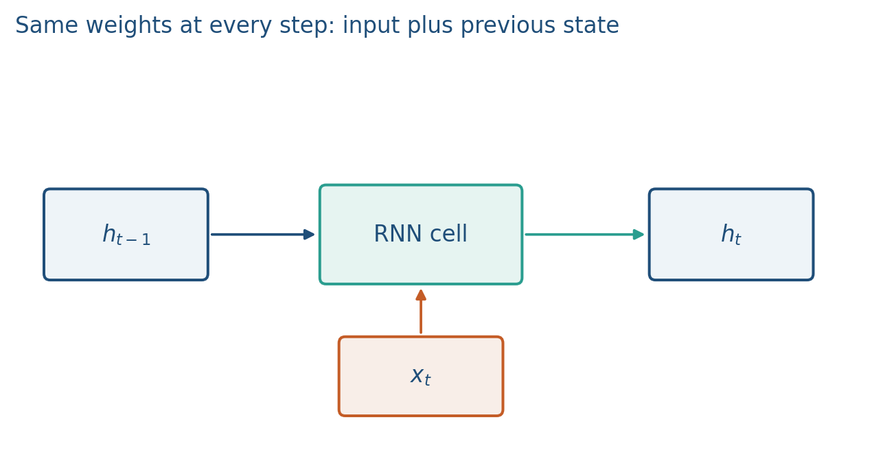
The vanilla (Elman) recurrence is

The same $W_h,W_x,\mathit{b}$ are used at every step. That is weight sharing along time, the sequence analogue of a CNN’s shared filter. An RNN language model then predicts the next token from ${\mathit{h}}_t$ with a linear map and a softmax.

Between two independent sequences (two reviews in a batch) you reset ${\mathit{h}}_0=\mathbf{0}$. The loop lives inside one sequence. If you do not reset, review 2 starts with leftover sentiment from review 1. That is leakage, not transfer learning.

2. Why we use it

A language model predicts the next token. Week 1 already wrote

An n-gram approximates the history by the last $n-1$ words and counts. Raise $n$ and the table is sparse; most strings never occurred. A fixed-window MLP concatenates the last $k$ embeddings and is dense, but $k$ is still a hard cutoff and each position in the window has its own weights. A bag of words cannot count “the verb agrees with the noun 40 tokens back” without growing width.

You need a map that (i) accepts any length, (ii) shares weights across time, and (iii) can, in principle, use the beginning of the sentence. That map is a recurrent cell.

Do not build an n-gram this week. The counting story is only here so the cell has a job.

3. Architecture

Write the loop as a chain. Four tokens, one set of weights:

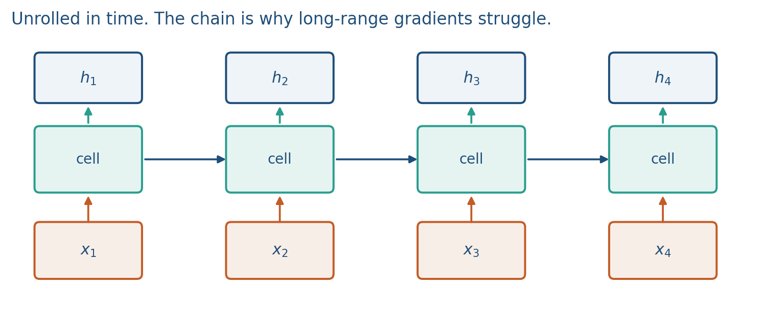
A CNN looks at a fixed neighborhood, in parallel. An RNN looks at everything so far, in order, and cannot fully parallelize across time. That is the accuracy / speed tradeoff.

Unrolling is how you backprop (note 2.2). The picture is one graph with copies of $W_h$. There are not four different matrices named $W_h^{(1)},W_h^{(2)},W_h^{(3)},W_h^{(4)}$.

If the first word is the subject of a verb twenty tokens later, ${\mathit{h}}_t$ must still contain that subject. The cell is a lossy compressor: every step overwrites. Week 2.2 is what happens to the gradient on that long path. Week 2.3 adds gates so the cell can choose what to keep.

The same cell, different wiring:

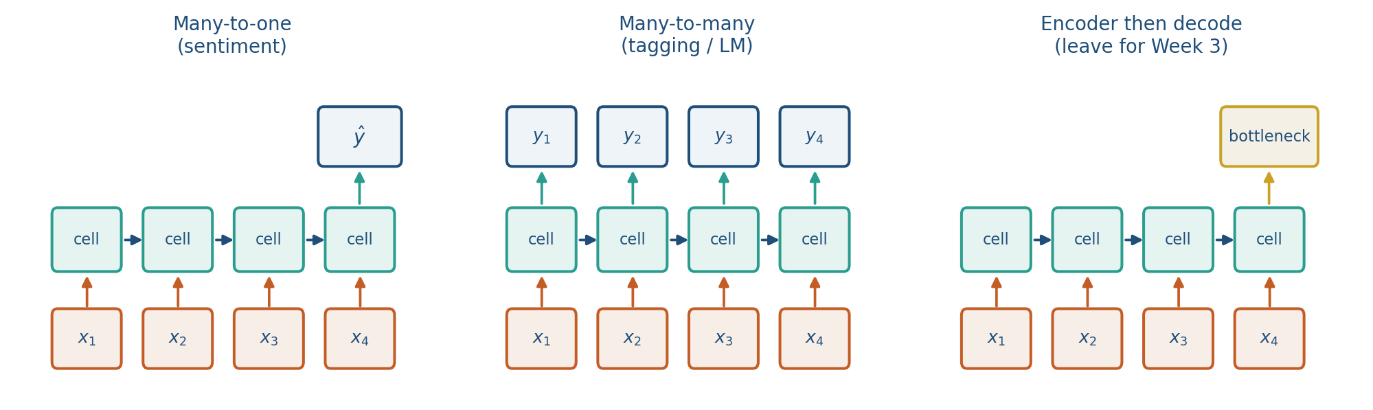
• Many-to-one (sentiment): read $x_1,\dots ,x_T$, emit from the last ${\mathit{h}}_T$. Lab 2 is this shape: copy the first bit at the end.
• Many-to-many, aligned (tagging, language modeling): emit at every $t$.
• Encoder then decode: compress the source into one vector, then generate. That bottleneck is why Week 3 exists. Do not train seq2seq this week.

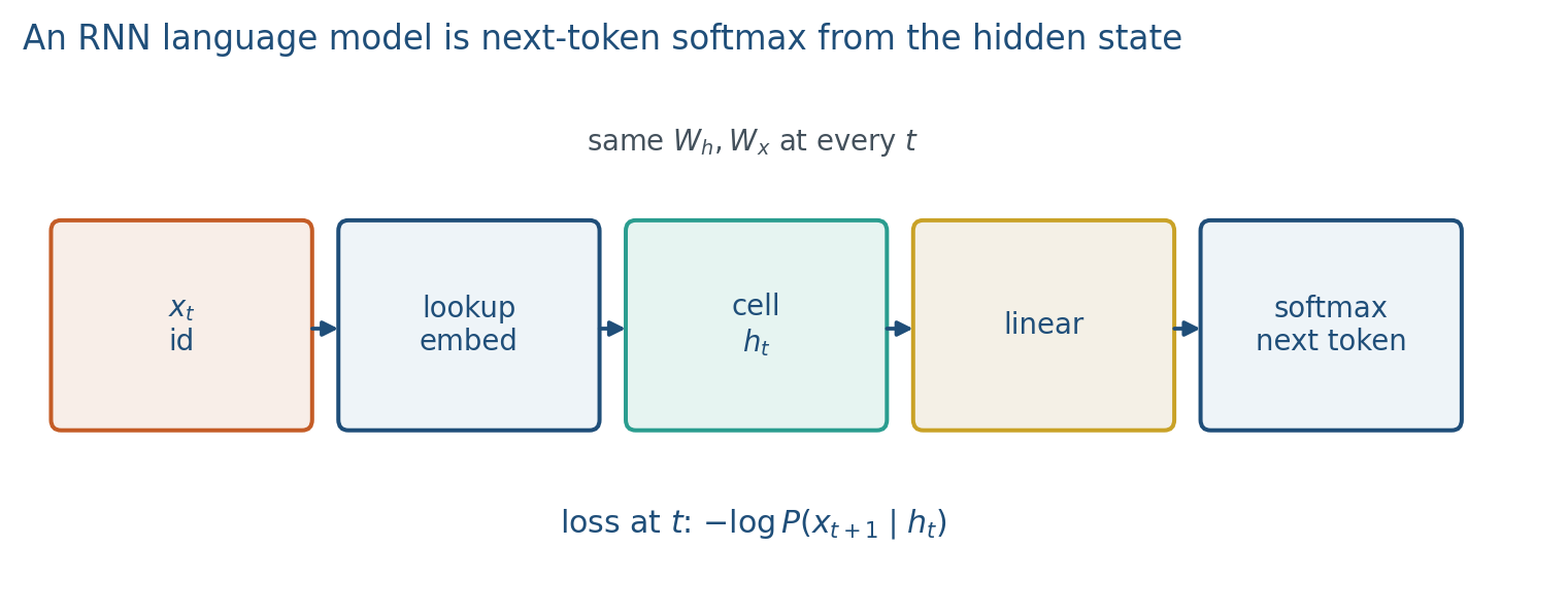
An RNN language model looks up the token id, runs the cell, then a linear map plus softmax over the vocabulary.

4. How it works, step by step

Read left to right. The same $W$ at every step.

1. Reset ${\mathit{h}}_0=\mathbf{0}$ at the start of the sequence.
2. Lookup ${\mathit{x}}_t$, mix it with ${\mathit{h}}_{t-1}$ through the shared cell, apply $\tanh$, get ${\mathit{h}}_t$.
3. For language modeling, map ${\mathit{h}}_t$ to vocabulary logits and take a softmax. The loss at step $t$ is the same next-token NLL as Week 1:

4. Average over tokens in the sentence (or a small batch of sentences). That is teacher forcing: the true previous token is the next input, not the model’s sample.

Perplexity is $\exp (\text{mean NLL})$ in nats, or $2^{\text{mean NLL}}$ if you used log base 2. Lower is better. You will not chase a Wikipedia perplexity number this week. You will chase whether Lab 2’s first bit is still in ${\mathit{h}}_T$.

Generation (optional picture): sample ${\widehat{x}}_{t+1}$ from the softmax, feed it back as $x_{t+1}$. Training does not do that.

A numeric two-step unroll is in the worked example. The teaser you should already see: token 1’s footprint in ${\mathit{h}}_2$ shrinks. That shrinkage is vanishing gradients, next note.

5. Mathematical formulas

The cell:

The joint factorization of a sequence, which the RNN-LM approximates by conditioning on ${\mathit{h}}_t$ instead of the raw history:

Next-token loss at step $t$:

Perplexity is $\exp (\text{mean NLL})$ in nats (or $2^{\text{mean NLL}}$ in bits). Lower is better.

6. Positive points and negative points

Positive.

• Variable length: one cell, any $T$, without growing a new table of n-grams.
• Parameter sharing across time is the sequence analogue of a CNN’s shared filter.
• In principle the state can carry the beginning of the sentence, which a fixed window cannot.
• The same cell wires as many-to-one (Lab 2) or many-to-many (language modeling).

Negative.

• Sequential: you cannot fully parallelize across time, unlike a transformer.
• The cell is a lossy compressor. Every step overwrites, so early tokens shrink in later states.
• Vanishing and exploding gradients on the unrolled chain (next note) kill long-range learning.
• Forgetting to reset $\mathit{h}$ between batch items leaks one document into the next.
• Training uses teacher forcing; sampling during training is not the RNN-LM loss.

When not to. If you need every token to see every other token in one hop, this is the wrong mixing layer. That is Week 3. This week you need the recurrent picture so the Jacobian product has somewhere to live.

7. Teaching this note

~18 minutes. Why a window is not enough, then the cell, then unroll three tokens with shared $W_h$, then the 2-D numeric table, then the RNN-LM diagram so next-token NLL has a hidden state. Play 0:00–12:00 of StatQuest RNNs (the loop and the unroll). Save vanishing gradients for note 2.2 even if the video teases them.

8. Worked example

Let $d=2$, $\mathit{b}=\mathbf{0}$, ${\mathit{h}}_0=\mathbf{0}$,

Step 1: $W_h{\mathit{h}}_0+W_x{\mathit{x}}_1={\mathit{x}}_1$, so ${\mathit{h}}_1=\tanh ({\mathit{x}}_1)\approx \left[\begin{array}{c}0.76\\ 0\end{array}\right]$ because $\tanh (1)\approx 0.76$.

Step 2: $W_h{\mathit{h}}_1+W_x{\mathit{x}}_2\approx \left[\begin{array}{c}0.38\\ 1\end{array}\right]$, then ${\mathit{h}}_2=\tanh (·)\approx \left[\begin{array}{c}0.36\\ 0.76\end{array}\right]$.

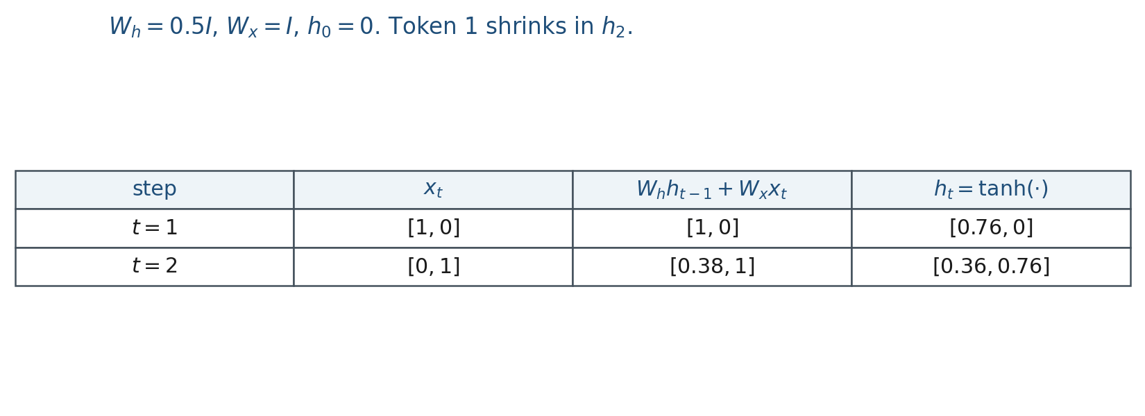
The same $W_h$ was used twice. Token 1 still has a shrunk footprint in ${\mathit{h}}_2$ ($0.76\to 0.36$). That shrinkage is the teaser for vanishing gradients.

9. Where students get stuck

• Drawing a new $W_h$ at each time step (no sharing).
• Feeding the whole sentence as one concatenated vector “to make it an MLP.”
• Forgetting to reset $\mathit{h}$ between batch items.
• Thinking an RNN-LM samples during training. It uses the true previous token.

10. Video

Watch StatQuest: Recurrent Neural Networks, Clearly Explained.

Pause on the first unroll (same weights copied) and on the moment the hidden state is described as memory. Skip any long software demo; the board math is the point.

11. Practice

1. Unroll three tokens on paper with $d=2$, ${\mathit{h}}_0=\mathbf{0}$. Which matrices are reused?

2. Why reset the state between two unrelated documents in a batch?

3. Name one thing an RNN can mix that a kernel of size 5 cannot, in a single layer.

4. Using the worked example’s $W_h,W_x$ and ${\mathit{x}}_3=\left[\begin{array}{c}1\\ 1\end{array}\right]$, write the pre-activation $W_h{\mathit{h}}_2+W_x{\mathit{x}}_3$ with ${\mathit{h}}_2\approx \left[\begin{array}{c}0.36\\ 0.76\end{array}\right]$. Do not bother with $\tanh$ if you are short on time; the linear mix is the lesson.

5. If every $W_h$ were replaced by $0.1I$, and ${\mathit{x}}_t=\mathbf{0}$ after $t=1$, approximately how does $\Vert {\mathit{h}}_t\Vert$ scale with $t$? (Geometric sequence.)

6. In one sentence: what is the loss at step $t$ of an RNN language model? What is teacher forcing?

7. Many-to-one or many-to-many: which wiring is Lab 2, and which wiring is next-token language modeling?