7.1 Scaling Laws

DATA 443/643 · Week 7 · PDF · Slides

Kaplan power laws, then Chinchilla: GPT-3 was 1.7 tokens/parameter, not 20.

These notes match the lecture slides. Use (slides) on the course hub for the deck.

Bigger models, trained on more data with more compute, tend to get better at next-token prediction. Scaling laws make that trend a curve you can fit, not a slogan. They do not promise a better chatbot; they promise a lower pretraining loss if the recipe stays the same.

1. What a scaling law is

A scaling law is a fitted curve of pretraining cross-entropy versus scale. You plot loss against compute $C$, parameter count $N$, or dataset size $D$, and you ask whether the cloud of runs looks like a smooth power law plus a floor. It is an empirical regularity for a fixed architecture family and a fixed data mixture, not a theorem that the next chatbot will be more helpful.

Kaplan et al. (2020) fit language-model loss against compute (and against $N$ and $D$) and saw smooth power laws over many orders of magnitude:

The irreducible term $L_{\infty }$ is entropy of the data plus whatever the architecture cannot represent. The interesting bit is the slope $-b$: extra FLOPs still buy loss, with diminishing returns. Once measured loss sits on $L_{\infty }$, the curve has already told you that more compute will not move the number.

Hoffmann et al. (2022), Chinchilla, asked a different question with the same ingredients. At a fixed FLOP budget, how should you split compute between a larger net and a longer token stream? Their fit said you should scale tokens and parameters together, not dump the budget into a huge model that sees the data once. The rule of thumb from that paper is about 20 tokens per parameter for the models they trained. Put it on the board as a rule of thumb from one paper, not a law of nature.

A scaling law is therefore two claims at once. Kaplan: loss versus scale looks like a power law plus a floor. Chinchilla: at fixed FLOPs, grow $N$ and $D$ together. Neither claim is “we trained a 7B.”

2. Why we use it

“We trained a 7B” is not a complete sentence. You need the token budget and whether you were compute-optimal. A smaller model trained longer can beat a larger undertrained one. That is why later LLaMA-style recipes look “small” next to GPT-3 and still read well: they were fed more tokens.

Early GPT-3-style runs were compute-optimal for a short training budget that underused data: a large $N$, not enough tokens. GPT-3 was $175B$ parameters on $300B$ tokens, about $1.7$ tokens per parameter. Chinchilla’s thumb is nearer $20$. A $70B$ model trained with enough tokens beat much larger undertrained nets.

You use the curve to plan a run. Fix two of $\{N,D,C\}$ and the third is constrained. Kaplan-style runs often oversize $N$ for a short $C$: the compute is spent on a wide net that barely sees $D$. Chinchilla re-spends that $C$ on more tokens. Same FLOP budget, different $(N,D)$. Write both numbers, not only “7B.”

A 7B model at 20 tokens/parameter wants about $7\times {10}^9\times 20=1.4\times {10}^{11}$ tokens. If you only have 14B tokens, you are 10$\times$ short of that rule of thumb—not “we scaled.” Lab 7 will fit $L=a{C}^{-b}+c$ on constructed points so you see the algebra, not a GPU cluster.

3. Architecture

This is not a new network. The object on the board is a log–log plot and a recipe $(N,D,C)$. The transformer is whatever you already had; the method is how you choose its size and its token budget.

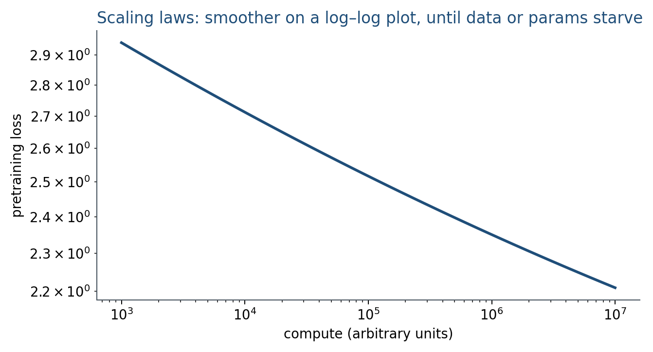
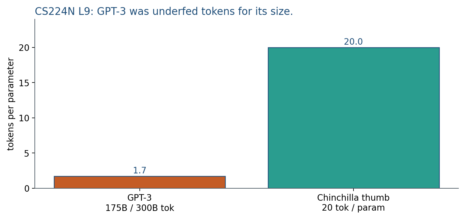
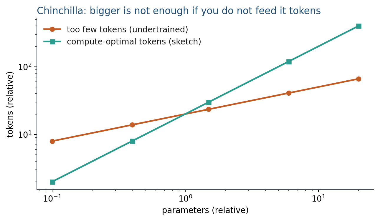
On the Kaplan plot, the x-axis is compute and the y-axis is pretraining loss. The curve falls, then flattens toward $L_{\infty }$. On the Chinchilla picture, two models sit at the same FLOP budget: one is wide and starved of tokens; the other is smaller and fed more data. The second is the balanced pair. Training FLOPs scale roughly as $6ND$ (forward plus backward), so holding $C$ fixed really does mean holding the product $ND$ fixed while you trade $N$ against $D$.

4. How it works, step by step

You do not train a new layer. You fit a curve, then you do arithmetic that makes “7B” a pair of numbers.

1. Collect runs (or, in Lab 7, constructed points) of pretraining loss versus compute. The range in the papers is many orders of magnitude; four noisy toy points are for the algebra.
2. Fit $L\approx a{C}^{-b}+L_{\infty }$. Read $b$ as diminishing returns and $L_{\infty }$ as the floor you cannot train through.
3. Name the budget. Training FLOPs cartoon: $\approx 6ND$. If you double $N$ and halve $D$, $C$ is unchanged.
4. Apply Chinchilla arithmetic. A 7B model at 20 tokens/parameter wants $7B\times 20=140B$ tokens. GPT-3’s $175B$ on $300B$ tokens is about $1.7$ tokens per parameter: oversized $N$ for that $C$.
5. Write both numbers in a report: checkpoint size and token budget. Two extra epochs on a toy set is not a scaling law.

Same FLOPs, two recipes. Model A: $N=4N_0$, $D=D_0/4$. Model B: $N=N_0$, $D=D_0$. Same $ND$. Chinchilla picks the balanced pair, not the 4$\times$-larger starved model. If the rule of thumb is 20 tokens/parameter, B matches it when $D_0=20N_0$; A has only 5 tokens/parameter.

5. Mathematical formulas

Kaplan’s compute law:

Lab 7 writes the same fit as $L=a{C}^{-b}+c$ on constructed points. The slope $-b$ is diminishing returns; $L_{\infty }$ (or $c$) is the floor.

Training FLOPs, cartoon:

Chinchilla’s planning thumb, from that paper’s fit, is about 20 tokens per parameter:

A 7B model then wants $7\times {10}^9\times 20=1.4\times {10}^{11}$ tokens. GPT-3’s ratio was $300B/175B\approx 1.7$. You do not need the papers’ full tables of $a$ and $b$ this week. You need to write $L(C)$, mark $L_{\infty }$, and compute a token budget at fixed $N$.

6. Positive points and negative points

Positive.

• A scaling law turns “bigger is better” into a curve you can fit and a recipe $(N,D,C)$ you can plan against.
• Chinchilla arithmetic stops “we trained a 7B” from being a complete sentence: you also write the token budget.
• Same FLOP budget, different $(N,D)$: a smaller model trained longer can beat a larger undertrained one.
• Lab 7’s toy fit shows the algebra of $a{C}^{-b}+c$ without a cluster.

Negative.

• $L$ is pretraining cross-entropy, not chat quality. Downstream accuracy is not $L$.
• Alignment (Weeks 8–9), data quality, mixture, and context length all sit off the curve.
• Inference cost still scales with $N$ even if you already paid for training.
• Four noisy toy points are not a law. The papers’ range is many orders of magnitude.
• The 20 tokens/parameter figure is a rule of thumb from one paper, not a law of nature.

When not to. Do not claim “we scaled” because you trained two extra epochs on a toy set. If your measured loss already sits on $L_{\infty }$, extra FLOPs buy almost nothing; change data or architecture instead of buying more compute.

7. Teaching this note

About 35 minutes at the board: write $L(C)$, mark $L_{\infty }$, then a Chinchilla arithmetic example (tokens vs parameters at fixed FLOPs). Play Karpathy after 20:00, especially 25:43–27:43 (scaling laws, ~2 min, plus a little context). The fit in Lab 7 is later in the week.

Put 20 tokens/parameter on the board as a rule of thumb from one paper, not a law of nature. Then do the 7B $\times$ 20 arithmetic so “we trained a 7B” is never a complete sentence.

8. Worked example

Suppose $L=2C^{-0.15}+1.4$. At $C={10}^4$,

At $C={10}^6$, ${10}^{-0.9}\approx 0.126$, so $L\approx 2·0.126+1.4=1.65$. A 100$\times$ compute jump bought $0.25$ nats, not a new architecture. If your measured loss is already $1.42$, you are sitting on $L_{\infty }$: extra FLOPs buy almost nothing.

Chinchilla, same FLOPs. Training FLOPs scale roughly as $6ND$ (forward+backward). Model A: $N=4N_0$, $D=D_0/4$. Model B: $N=N_0$, $D=D_0$. Same $ND$. Chinchilla picks the balanced pair, not the 4$\times$-larger starved model. If the rule of thumb is 20 tokens/parameter, B matches it when $D_0=20N_0$; A has only 5 tokens/parameter.

9. Where students get stuck

• Reading $L$ as “chat quality.” It is pretraining cross-entropy.
• Thinking a bigger $N$ always wins at fixed FLOPs. Chinchilla is the counterexample.
• Fitting $a,b,c$ on four noisy toy points and claiming a law. Lab 7 is the algebra; the paper’s range is many orders of magnitude.

10. Video

Karpathy — Intro to Large Language Models. Play from 20:00, and pause on 25:43–27:43 (scaling laws). The first 20 min were Week 1; this hour is the compute curve and why tokens matter as much as parameters.

11. Practice

1. Two models, same FLOPs. One has $4\times$ the parameters and $1/4$ the tokens of the other. Who does Chinchilla pick, and why?

2. If $L_{\infty }$ is already almost your measured loss, what does extra compute buy?

3. Why can a scaling law look great while a chat eval is flat?

4. Using $L=2C^{-0.15}+1.4$, compute $L$ at $C={10}^5$. (${10}^{-0.75}\approx 0.178$.)

5. A 1B-parameter model trained on 4B tokens. Using 20 tokens/parameter, is it over- or under-trained on data? By what factor?