9.1 Preference Data and Reward Models

DATA 443/643 · Week 9 · PDF · Slides

Bradley–Terry on a pair. Chance is log 2. Best-of-n uses the RM without PPO.

These notes match the lecture slides. Use (slides) on the course hub for the deck.

SFT copies demonstrations. Preferences say which of two replies is better when both are fluent. A reward model (RM) is a classifier of that comparison. Week 9.2 will use the RM inside RL; Week 9.3 will skip it.

1. What a reward model is

A human (or a strong teacher model) sees a prompt $x$ and two completions $y_w$ (chosen, winner) and $y_l$ (rejected, loser). The label is a pairwise order, not a numeric grade. Ties and multi-way ranks exist; this course uses pairs. A reward model (RM) is a scalar scorer $r_{\varphi }(x,y)$ trained so that the chosen reply gets a higher number than the rejected one.

Bradley–Terry turns that comparison into a logistic: the probability that $y_w$ beats $y_l$ is $\sigma (r(x,y_w)-r(x,y_l))$. The loss is $-\log$ of that probability. Only differences enter. $r_{\varphi }$ is not a grade out of 10, not truth, and not “helpfulness” in the abstract. It is a fit to the raters you hired, on the prompts you wrote.

If the two rewards are equal, the argument of $\sigma$ is 0 and $\sigma (0)=1/2$, so the loss is $\log 2\approx 0.693$. That is chance: the RM has not ordered the pair. Lab 9 will fit this on toy scores.

2. Why we use it

SFT copies a single answer. Preferences say “this is better than that” without writing a scalar label by hand. It is easier to compare than to write, which is why we collect pairs, not essays.

A base LM that already speaks still needs a way to rank two fluent replies. The RM is that ranker. At test time you can rank $n$ samples from the policy by $r_{\varphi }$ (best-of-$n$) without any RL. Best-of-$n$ already uses this RM and is a competitive baseline (AlpacaFarm). It is not PPO. You sample $n$ from SFT and return the RM’s favorite. PPO (next note) trains a new ${\pi }_{\theta }$.

Collection is the bottleneck: instructions must be clear, raters disagree, and the pair set can encode rater bias. If both $y_w$ and $y_l$ are wrong, the RM still learns a relative order among mistakes. Held-out preference accuracy—how often $r_{\varphi }(x,y_w)>r_{\varphi }(x,y_l)$ on pairs the RM did not train on—is the number to report. Do not report only training loss.

3. Architecture

Initialize from the SFT policy (or its encoder). The RM already speaks the same dialect as the completions it must score. A raw pretrained LM does not format like an assistant, so its scalar head starts on the wrong geometry.

Usually you keep the base LM and add a scalar head on the last token, or you train a small classifier that reads the completion. There is no PPO loop in this note. Best-of-$n$ is the serve-time architecture: sample $n$, pick $\mathrm{\backslash arg}maxr$.

Δ values and the logistic loss" src="files/graphics/9.1-preference-rewards/rm-numeric.png" />

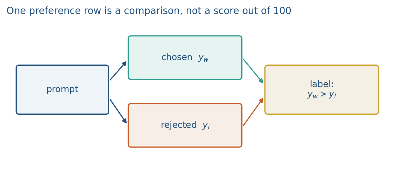
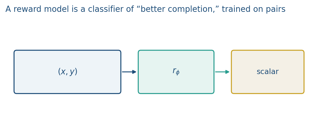
The picture is a pair in, a difference of scalars, a logistic loss. Lab 9 is a tiny head on toy scores so you can print $\Delta$ and $\sigma (\Delta )$ without an LLM.

4. How it works, step by step

1. Collect pairs. Prompt $x$, chosen $y_w$, rejected $y_l$. Clear instructions to raters; expect disagreement.
2. Initialize $r_{\varphi }$ from SFT. Score each completion with a scalar.
3. Train the Bradley–Terry / logistic loss below. Chance loss is $\log 2$. Large positive $\Delta$ $\to$ loss near 0; large negative $\Delta$ (chosen scored below rejected) $\to$ loss near $\infty$.
4. Check held-out accuracy, not only train loss. The RM is a pairwise logistic classifier, not a calibrated “helpfulness out of 10.”
5. Optional decode: best-of-$n$. Sample $n=8$ completions from ${\pi }_{\mathrm{S}\mathrm{F}\mathrm{T}}$, score each with $r_{\varphi }$, return $\mathrm{\backslash arg}{max}_i{r}_{\varphi }(x,y_i)$. Extra cost: 8 policy forwards plus 8 RM forwards (the RM is usually cheaper). No PPO. The distribution is “SFT, then pick the RM’s favorite,” not a new ${\pi }_{\theta }$. If two samples share the top score, freeze a tie-break (lower id, or a second sample) so a demo is reproducible; the RM failed to separate them.

Reward hacking waits in the next notes: the policy learns to please $r_{\varphi }$ with verbose, sycophantic, or empty-safe text. That is why RLHF adds a KL penalty to the SFT model, and why you keep a held-out preference set.

5. Mathematical formulas

Bradley–Terry probability and RM loss:

$\sigma (\Delta )=(1+e^{-\Delta }{)}^{-1}$. If $r_w=r_l$, $\Delta =0$, $\sigma (0)=1/2$, ${ℒ}_{\text{RM}}=\log 2\approx 0.693$ nats per pair.

Worked numbers live in the example below: $\Delta =2$ gives $\sigma \approx 0.881$ and loss $\approx 0.127$; a flipped pair $\Delta =-2$ gives loss $\approx 2.13$. Compute $\log 2$ once as a class so “0.693 at init” is a number people can check in Lab 9, not a magic constant.

6. Positive points and negative points

Positive.

• Pairwise data is easier to collect than absolute scores or full essays.
• The same RM already gives a strong decode baseline: best-of-$n$, no PPO.
• Init from SFT puts the scalar head on assistant-shaped text.
• Held-out preference accuracy is a number you can rerun after a policy update.

Negative.

• Reward hacking: a later policy can please $r_{\varphi }$ with verbose, sycophantic, or empty-safe text.
• RM error becomes policy error. A relative order among two wrong answers is still an order.
• Best-of-$n$ spends compute at decode ($n$ policy forwards plus $n$ RM forwards).
• $r_{\varphi }$ is not truth or safety in the abstract; it is a fit to your raters and prompts.
• Reporting only training loss hides a held-out accuracy that never left chance.

When not to. Do not call best-of-$n$ “RLHF.” It uses the RM; it does not train a policy with PPO. If you have no preference pairs, you do not have an RM—you have SFT.

7. Teaching this note

About 30–35 minutes at the board: one pair, write $\sigma (\Delta r)$, compute $\sigma (0)$, then best-of-$n$ cost. Play Karpathy’s RLHF / comparison appendix 21:05–25:43. Lab 9 section 1 is the toy logistic RM.

Compute $\log 2$ once as a class so “0.693 at init” is a number people can check in Lab 9, not a magic constant.

8. Worked example

Rewards $r_w=2.0$, $r_l=0.0$. Difference $2$. $\sigma (2)=1/(1+e^{-2})\approx 0.881$. Loss $-\log 0.881\approx 0.127$.

If $r_w=r_l=1.7$ always, $\Delta =0$, $\sigma (0)=1/2$, $ℒ=-\log (1/2)=\log 2\approx 0.693$ nats per pair. A random RM sits here.

Best-of-$n$: sample $n=8$ completions from ${\pi }_{\mathrm{S}\mathrm{F}\mathrm{T}}$, score each with $r_{\varphi }$, return $\mathrm{\backslash arg}{max}_i{r}_{\varphi }(x,y_i)$. Extra cost: 8 policy forwards plus 8 RM forwards (the RM is usually cheaper). No PPO. The distribution is “SFT, then pick the RM’s favorite,” not a new ${\pi }_{\theta }$.

Init from SFT: the RM already speaks the same dialect as the completions it must score. A raw pretrained LM does not format like an assistant, so its scalar head starts on the wrong geometry.

If $r_w=0$, $r_l=2$, $\Delta =-2$, $\sigma (-2)\approx 0.119$, loss $-\log 0.119\approx 2.13$. The RM is wrong on that pair; that is a large gradient. Lab 9 should print both the easy pair and a flipped pair.

9. Where students get stuck

• Treating $r_{\varphi }$ as a grade out of 10. Only differences enter the loss.
• Forgetting $\sigma (0)=1/2$ when the two rewards match.
• Calling best-of-$n$ “RLHF.” It uses the RM; it does not train a policy with PPO.

10. Video

Karpathy — Intro to Large Language Models. Play the RLHF / preference section 21:05–25:43 (comparisons, labeling, RLHF). Pause on “it is easier to compare than to write”: that is why we collect pairs, not essays. PPO details wait for note 9.2.

11. Practice

1. If $r(x,y_w)=r(x,y_l)$ always, what is ${ℒ}_{\text{RM}}$?

2. Why initialize the RM from SFT instead of from a raw pretrained LM?

3. Best-of-$n$ uses the RM without PPO. What extra cost did you pay at inference?

4. Compute $\sigma (r_w-r_l)$ and the RM loss for $r_w=1$, $r_l=-1$. ($\sigma (2)\approx 0.881$.)

5. You score $n=4$ samples. Two share the top RM score. How do you break the tie in a reproducible demo, and what did the RM fail to do?