11.3 Mode Collapse and Evaluation

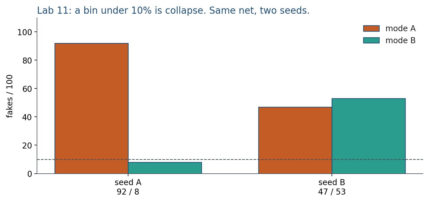
92/8 is collapse. 47/53 is covered. G’s loss has no missing-mode term.

These notes match the lecture slides. Use (slides) on the course hub for the deck.

A GAN has no likelihood you can read as “this model covers the data.” The usual failure is not blur. It is mode collapse: the generator finds one (or a few) fakes that fool $D$ and repeats them. By the end you should be able to tell fidelity from coverage, apply Lab 11’s binning rule, and explain why a healthy $G$ loss does not rescue a missing mode.

1. What mode collapse is

Mode collapse is when $G$ parks on a few modes and $D$ is still happy. Each fake can look fine. The set of fakes does not. One pretty sample is not a trained $G$ .

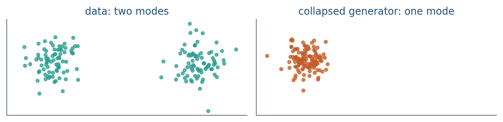
Suppose the reals are two well-separated clusters. If $G$ parks all of its mass on cluster A, $D$ learns “cluster A might be fake; cluster B is real.” $G$ then jumps to B. You cycle. Or $G$ never leaves A, and every sample looks plausible while half the world is missing.

This is the 1-D spike example from note 11.1 with motion. $D$ only needs to be wrong on the support of $G$ . Modes that $G$ never visits do not appear in $G$ ’s loss at all. There is no extra term in vanilla $J$ that says “visit mode 2.” That is the bug.

On Lab 11’s two Gaussians, 92/8 is collapse (or heavy imbalance). 47/53 is covered. Same architecture, different outcome. That is why you report the bin fractions, not only lossG.

2. Why we use it

You study collapse because it is the evaluation lesson of Week 11, not a rare pathology. $D$ only scores “is this fake?” It does not have a missing-mode term. $G$ can fool $D$ with one spike, collect a small generator loss, and still miss half the data.

Eyeballing a grid of images checks fidelity (does this one look real?). It does not check whether you missed a mode. GANs stay useful for fast sampling. Diffusion (Week 12) is slower and usually covers better, which is why text-to-image moved there. The evaluation lesson does not move: always measure the mode you might have dropped.

For a project, write the coverage check before you train. “The pictures look nice” is not a metric.

3. Architecture

The architecture is the same GAN as notes 11.1 and 11.2. What changes is what you measure. Evaluation needs bins / modes, not only ${l o s s}_{G}$ .

Two numbers belong in a report:

Question	Informal name
Are the fakes realistic?	precision / fidelity
Did we hit the real support?	recall / coverage

On images, people cite FID or precision–recall in Inception space. Those are proxies. They need a large sample, and they inherit the classifier’s biases. On Lab 11 you can skip Inception: count how many fakes fall near each Gaussian mean.

A coverage statistic for two modes: assign each fake to the nearest mean, report the two fractions. Lab 11 calls it collapse if either bin is under $10 %$ . Write both percentages in the report even when they look like $48 / 52$ : that is the evidence, not a screenshot of two clouds.

Latent interpolations are a third check. A short step in $z$ should change the sample a little. A jump from “shoe” to “face” is a symptom of a broken map, not a feature. You will not train StyleGAN here; you will print two bin fractions.

4. How it works, step by step

Lab 11 is two 1-D Gaussians in 2-D clothing: means $μ_{A} = (- 2, 0)$ and $μ_{B} = (2, 0)$ . Collapse is visible because the mixture is simple.

Train the GAN as in note 11.2. Do not stop when ${l o s s}_{G}$ looks small.
Draw a large batch of fakes (the worked example uses 100).
Assign each fake to the nearest mean by Euclidean distance.
Report the two fractions. If either bin is under $10 %$ , write collapse (or heavy imbalance) by the lab rule.
Read $D$ on the parked mode versus the missing mode. If $D (G (z)) \approx 0.5$ on A and $D \approx 0.99$ on B, $G$ is paid for staying on A. Nothing in $J$ pulls it toward B.

Fixes are habits, not a single switch: do not let $D$ become perfect; try more noise dimensions; unrolled or Wasserstein losses in a later paper; mixture data in the lab so collapse is visible. Switching to diffusion (Week 12) is a different family with better typical coverage, not a GAN hyperparameter.

5. Mathematical formulas

Vanilla $J$ is still

J = 𝔼_{x ~ p_{r}} [\log D (x)] + 𝔼_{z ~ p_{z}} [\log (1 - D (G (z)))] .

There is no extra loss term that says “visit mode 2.” If $p_{G}$ puts no mass on a real cluster, that cluster never appears in the second expectation, so $G$ is not penalized for missing it.

For two modes, the coverage fractions after nearest-mean assignment of $N$ fakes are

{\hat{π}}_{A} = \frac{n_{A}}{N}, {\hat{π}}_{B} = \frac{n_{B}}{N} .

Lab 11 flags collapse when $min ({\hat{π}}_{A}, {\hat{π}}_{B}) < 0.10$ .

6. Positive points and negative points

Positive.

Collapse is easy to demo on two Gaussians: you can count, you do not need Inception.
The fidelity-versus-coverage split is the right report structure for any implicit generator, including later diffusion samples.
Lab 11’s $10 %$ rule gives a yes/no you can write next to the two fractions.
Interpolation in $z$ is a cheap extra check that the map is not a bag of disconnected spikes.

Negative.

Image metrics (FID) are imperfect coverage proxies: they need a large sample and inherit a classifier’s biases.
Fixing collapse is still research-level; there is no single switch in this course.
Generator loss can look healthy while half the clusters have no fakes.
Averaging FID (or a 2-D MSE to the origin) across a collapsed cloud can look like a pass.

When not to treat collapse as “the pictures are bad.” Sharp and identical is collapse. Sharp and diverse is the goal. Diffusion if you need coverage more than one-pass speed.

7. Teaching this note

About 30 minutes at the board, then ~10 minutes of video. Lab 11 should start in this same class meeting.

0–10 min. Replay the two-spike cartoon. Collapse vs oscillation.
10–20 min. Fidelity vs coverage table. Write the Lab 11 binning rule on the board.
20–30 min. Worked count: 100 fakes, 92 / 8. Precision high, recall not.
Then play 64:00–74:00 of the assigned video (training is unstable; you do not have $p (x)$ ; samples can look good anyway). Pause on the summary and name that gap coverage.

8. Worked example

Lab 11 means: $μ_{A} = (- 2, 0)$ , $μ_{B} = (2, 0)$ . You sample 100 fakes. Euclidean nearest-mean assignment:

92 fakes closer to $μ_{A}$
8 closer to $μ_{B}$

Coverage fractions: $0.92$ and $0.08$ . The $8 %$ bin is under $10 %$ : collapse (or heavy imbalance) by the lab rule.

A human looking at the 92 points near A says they look like reals. Fidelity is high on A. Recall of the mixture is not.

Generator loss can still be small: $D$ only fights A, so $D$ on A drifts toward $0.5$ , and $G$ is paid for staying there. The 8 points on B are not a rescue; they are leftover jitter.

If a second seed gives 47 / 53, write covered. Same architecture, different outcome. That is why you report the bin fractions, not only lossG.

You can interpolate in $z$ when the map is healthy (StyleGAN made that famous). A jump from “shoe” to “face” is a broken map. You will not train StyleGAN here; you will print two bin fractions.

9. Where students get stuck

Equating “sharp samples” with a trained GAN. Sharp and identical is collapse.
Using $G$ ’s loss as a coverage metric. It has no term for missing modes.
Averaging FID (or a 2-D MSE to the origin) across a collapsed cloud and calling it a pass.

10. Video

Watch Generative models: coverage and collapse, 64:00–74:00.

Pause on instability and the recap that GANs do not give you $p (x)$ or inference queries. The lecture’s word is “unstable”; your word in this course is mode collapse / coverage. Same URL as 11.1 and 11.2.

11. Practice

Why can a generator loss look healthy while half the training clusters have no fakes?
High precision, low recall: what did the GAN do?
You have two 2-D Gaussians as reals. Write one coverage statistic you would print in Lab 11 that is not a loss.
200 fakes; 186 assigned to mean A, 14 to mean B. Do you write collapse under the lab’s $10 %$ rule? What are the two fractions?
$D (G (z)) = 0.48$ on every fake, all fakes sit on mode A, and $D = 0.99$ on mode B. Why is $G$ not pulled toward B?

Ahmad Mousavi