1.3 Gradient Descent

Forward, loss, backward, update, and one ReLU unit’s chain rule. That loop is pretraining.

These notes match the lecture slides. Use (slides) on the course hub for the deck.

Training a net is an optimization problem: pick weights so a loss is small on training batches, then check a held-out set. Gradient descent is the default way to move the weights. By the end you should be able to write the update, take two numeric steps on a parabola, and chain-rule one ReLU unit by hand.

1. What gradient descent is

Collect all weights and biases into one vector $θ$ . A loss $L (θ)$ is a scalar. Gradient descent repeatedly walks downhill on that surface: each step subtracts a scaled gradient. Stochastic gradient descent (SGD) estimates $\nabla L$ on a minibatch, not the full dataset. That is how nets learn, including the pretraining loop of a language model.

For classification the loss is often cross-entropy; for a regression toy it is squared error. In two dimensions you can draw the contours. Gradient descent follows $- \nabla L$ .

Gradient descent on a bowl-shaped loss

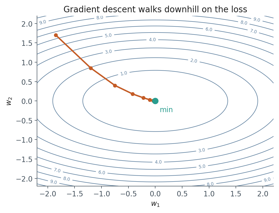
The picture is a cartoon. Real nets live in millions of dimensions. The geometry is still the same idea: the gradient is the direction of steepest increase, so you walk the other way.

Nielsen calls this the cost; the usual name here is loss; a statistician calls it empirical risk. Same object. You need one scalar, then one vector of derivatives.

2. Why we use it

You cannot solve $\nabla L = 0$ in closed form for a deep net. The training loop of pretraining is this walk, at huge batch and data scale. Fine-tuning (Week 8) is the same loop on a smaller, more specific dataset. RLHF (Week 9) changes what $L$ is, not the fact that you are differentiating a scalar with respect to weights.

Cross-entropy on a next-token distribution is the LLM default. For one token with predicted probability $p$ on the correct class,

L = - \log p .

If the gradient is noise, or $η$ is wrong, or the net is linear, no amount of later “prompt engineering” will save the representation. Get this loop right on a tiny problem in Lab 1 before you touch Hugging Face.

A noisy minibatch gradient is not a bug. It is the only gradient you can afford, and the noise can help you leave sharp spikes. The price is that one step is not guaranteed to decrease $L$ .

3. Architecture

One training iteration is four moves, in that order.

Forward. Compute activations layer by layer. Keep them; the backward pass needs them.
Loss. Compare $\hat{y}$ to the target $y$ .
Backward. Chain rule from the loss to every weight (backpropagation).
Update. Take a descent step on $θ$ .

The training loop

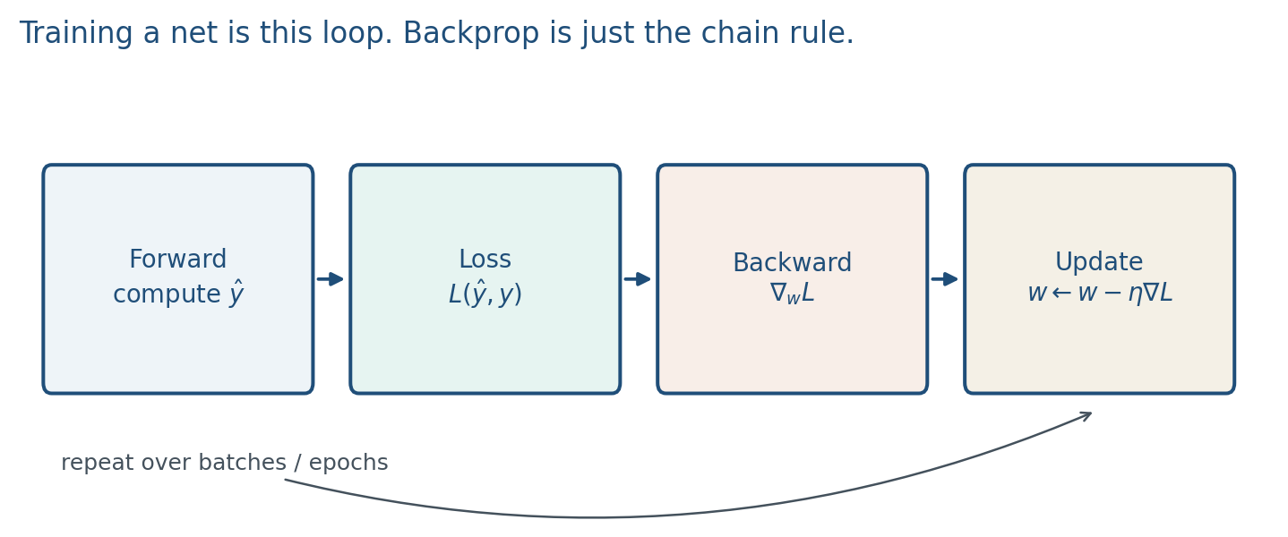
PyTorch does (3) for you if the forward pass used nn.Module and a differentiable loss. Your job is to write (1), pick $L$ , and call optimizer.step().

If you forget zero_grad(), gradients accumulate across steps. That is a silent $η$ disaster, not a new algorithm.

Adam and related methods rescale coordinates using a running average of gradients; you will use them in PyTorch without deriving them today. The architecture of the loop does not change: forward, loss, backward, update.

4. How it works, step by step

One step is

θ \leftarrow θ - η \nabla_{θ} L (θ) .

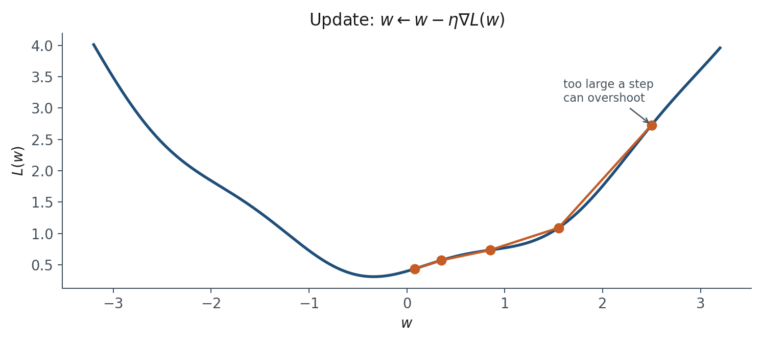
$η$ is the learning rate. Too small: you crawl. Too large: you jump over the valley or diverge.

A 1-D loss and a few descent steps

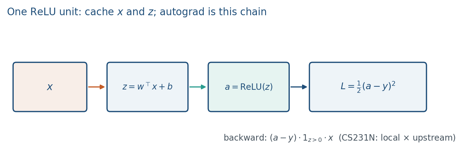
Treat each operation as a gate with a local derivative. Autograd is that picture. For squared error on one ReLU neuron,

z = w^{⊤} x + b, a = ReLU (z), L = \frac{1}{2} (a - y)^{2} .

Chain rule, using ${ReLU}^{'} (z) = 1_{z > 0}$ from note 1.2:

\frac{\partial L}{\partial w} = (a - y) {ReLU}^{'} (z) x .

Same pattern for $b$ , with $x$ replaced by $1$ . If $z \leq 0$ , the local derivative is 0 and that example does not move $w$ . That is a dead ReLU on this point, not a PyTorch bug.

One ReLU unit as a chain of gates

Lab 1 uses binary cross-entropy on logits $z$ , not on $σ (z)$ . PyTorch’s BCEWithLogitsLoss is

L = max (z, 0) - z y + \log (1 + e^{- | z |}),

which is numerically stable BCE. The extra line you need: pass $z$ , never sigmoid(z), into that loss. If you sigmoid first, you squash twice.

SGD uses a minibatch, not the full dataset. That is how you train on Wikipedia-scale text. We do not need Adam’s derivation this week.

5. Mathematical formulas

The descent step:

θ \leftarrow θ - η \nabla_{θ} L (θ) .

Next-token cross-entropy on the correct-class probability $p$ :

L = - \log p .

Chain rule on one ReLU unit with squared error $L = \frac{1}{2} (a - y)^{2}$ :

\frac{\partial L}{\partial w} = (a - y) {ReLU}^{'} (z) x = (a - y) 1_{z > 0} x .

The softmax/cross-entropy cousin is $\partial L / \partial w = (p - y) x$ . Same “upstream error times input” shape.

Stable binary cross-entropy on a logit $z$ (what BCEWithLogitsLoss computes):

L = max (z, 0) - z y + \log (1 + e^{- | z |}) .

6. Positive points and negative points

Positive.

The update is simple and scales to millions of steps on huge corpora.
Minibatch SGD is the gradient you can actually afford; the noise can help leave sharp spikes.
Autograd turns a forward graph of gates into the backward pass, so you write the net once.
The same loop is pretraining, fine-tuning, and (with a different $L$ ) RLHF.

Negative.

Local minima and saddles exist; a step is not guaranteed to decrease $L$ under minibatch noise.
$η$ is a choice: too small crawls, too large overshoots or diverges.
Forgetting zero_grad() silently accumulates gradients and wrecks the effective step size.
Passing sigmoid(z) into BCEWithLogitsLoss double-squashes and is a common Lab 1 bug.
If $z \leq 0$ on a ReLU unit, that example does not move $w$ ; dead units stay dead.

When not to. If you can solve $\nabla L = 0$ in closed form (a linear least-squares toy), do that. Deep nets are not that toy.

7. Teaching this note

~18 minutes. Draw a 1-D parabola, write the update, do two numeric steps plus the overshoot, then the four-box loop and zero_grad. Spend four minutes on the one-ReLU chain rule and the BCEWithLogitsLoss warning. 3Blue1Brown gradient descent (0:00–12:00) and the backprop follow-up are homework. Do not derive a softmax Jacobian in this block.

8. Worked example

Let $L (θ) = (θ - 3)^{2}$ , start at $θ_{0} = 0$ , take $η = 0.25$ . Then $\nabla L = 2 (θ - 3)$ .

Step 1:

θ_{1} = 0 - 0.25 \cdot 2 (0 - 3) = 0 - 0.25 \cdot (- 6) = 1.5 .

Step 2:

θ_{2} = 1.5 - 0.25 \cdot 2 (1.5 - 3) = 1.5 - 0.5 \cdot (- 1.5) = 2.25 .

The minimum is at $3$ . You moved $0 \to 1.5 \to 2.25$ . If you instead take $η = 2$ , step 1 is $0 - 2 \cdot (- 6) = 12$ , which overshoots. Draw both arrows on the same parabola.

One-unit check: $x = 2$ , $w = 0.5$ , $b = 0$ , $y = 1$ . Then $z = 1$ , $a = ReLU (1) = 1$ , $L = 0$ , so $\partial L / \partial w = 0$ . Change $y$ to $0$ : $a - y = 1$ , ${ReLU}^{'} (1) = 1$ , $\partial L / \partial w = 1 \cdot 1 \cdot 2 = 2$ . One SGD step with $η = 0.1$ sends $w \leftarrow 0.5 - 0.1 \cdot 2 = 0.3$ .

9. Where students get stuck

Walking up the gradient (forgetting the minus sign).
Thinking SGD is “wrong GD” rather than the scalable estimator of $\nabla L$ .
Dropping activations after the forward pass, then being surprised that backward needs them.
Passing sigmoid(z) into BCEWithLogitsLoss (the loss already includes the sigmoid).

10. Video

Watch 3Blue1Brown: Gradient descent, how neural networks learn.

Pause when the ball follows $- \nabla L$ , and when a large step jumps the valley. Optional: 3Blue1Brown: What is backpropagation really doing? after class (~14 min); pause on the chain-rule diagram, not the code.

11. Practice

You double $η$ and the loss oscillates. What happened geometrically?
Why keep $a^{(1)}$ after you already have $\hat{y}$ ?
SGD uses a minibatch. Name one reason that is not “the full gradient is too slow.”
For $L (θ) = θ^{2}$ , $θ_{0} = 4$ , $η = 0.1$ , write $θ_{1}$ and $θ_{2}$ . (Use $\nabla L = 2 θ$ .)
Same $L$ and $θ_{0} = 4$ , but $η = 1.1$ . Compute $θ_{1}$ . Did the step move closer to $0$ or farther?
For the one-ReLU unit with $x = 2$ , $w = 0.5$ , $b = 0$ , $y = 0$ , write $\partial L / \partial w$ . Then take $η = 0.1$ and the new $w$ .

Ahmad Mousavi