11.2 Training Dynamics

Minimax J. Non-saturating −log D(G(z)). A 99% D is often a dead G.

These notes match the lecture slides. Use (slides) on the course hub for the deck.

The two nets have opposite goals. You cannot treat a GAN as one ordinary loss. Each step is a small fight: first improve $D$ , then improve $G$ , and try not to let either win too hard. By the end you should be able to write $J$ , run the two-phase loop, and say why a 99% discriminator is a problem, not a trophy.

1. What GAN training is

GAN training is a min-max game, not a single supervised loss. $D$ wants to tell real from fake. $G$ wants to fool $D$ . Goodfellow et al. write that as ${min}_{θ_{g}} {max}_{θ_{d}} J (θ_{g}, θ_{d})$ . A Nash point you hope for is that $G$ matches the real distribution and $D$ is a coin flip. Training does not guarantee you land there.

Each iteration has two phases. First you improve $D$ on a batch of reals and fakes. Then you improve $G$ on fresh noise. The original saturating loss for $G$ is weak when $D$ is already sharp, so people use a non-saturating surrogate $- \log D (G (z))$ instead of minimizing $\log (1 - D (G (z)))$ .

You are not adding a KL term. That is RLHF, a different week. Here the only fight is $J$ , plus the surrogate $G$ actually climbs.

2. Why we use it

If you only train $D$ to 99%, $G$ gets no gradient: fakes are so obviously fake that $\log (1 - D (G (z)))$ sits near 0 and the slope with respect to $G$ vanishes. If you only train $G$ , $D$ is stale and becomes a noisy, lying teacher. The two parameter vectors have to stay in tension.

Watching $J$ is not evaluation. A falling generator loss can mean better fakes or a collapsing $D$ . You still have to look at samples and at coverage (note 11.3). Lab 11 is a 2-D version of this fight on purpose: you will see the tension in a scatter plot, not in a single scalar.

Learning rates, how many $D$ steps per $G$ step, and batch size all move that balance. The two nets can oscillate: losses look fine, then the samples jump.

3. Architecture

The architecture is the same two nets as note 11.1. What is new is the update rule: alternate (or simultaneous) SGD steps, with a freeze on the net you are not training.

Train $D$ . A batch of reals (label 1) and fakes from the current $G$ (label 0). Binary cross-entropy. Update only $θ_{d}$ . Detach the fakes so the $D$ step does not also move $G$ .
Train $G$ . Fresh noise, fresh fakes. Labels are all 1: you want $D$ to be wrong. Freeze $θ_{d}$ ; update only $θ_{g}$ .

Generator and discriminator losses pulling in opposite directions

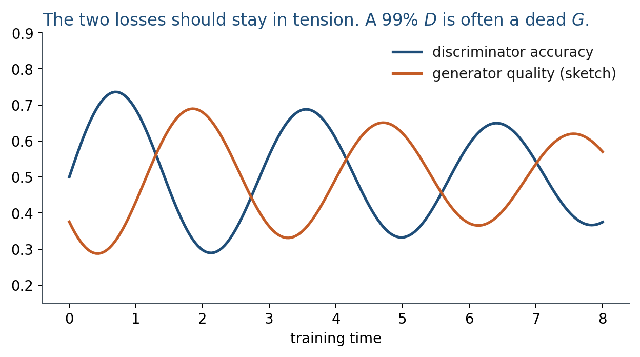
Lab 11’s loop is exactly this, with BCEWithLogitsLoss: one $D$ step, one $G$ step, 400 iterations. Print both losses. Do not rank checkpoints by the smaller number.

4. How it works, step by step

Read the two terms of $J$ out loud. First term: on reals, $\log D (x)$ is large when $D \approx 1$ . Second term: on fakes, $\log (1 - D (G (z)))$ is large when $D \approx 0$ . $G$ only appears in the second term, and it wants that term small, i.e. $D (G (z))$ near 1.

Sample a real batch and a noise batch. Form fakes $G (z)$ with the current generator.
Phase D. Maximize $\log D$ on reals plus $\log (1 - D)$ on fakes. Update only $θ_{d}$ .
Phase G. Draw fresh noise. In code you often maximize $\log D (G (z))$ instead of minimizing $\log (1 - D (G (z)))$ . Early in training $D$ is too good and the second form saturates: if $D (G (z)) \approx 0$ , then $\log (1 - D) \approx 0$ and the slope with respect to $G$ is tiny. $- \log D (G (z))$ still has slope.
Repeat. If $D$ is too weak, $G$ gets a noisy teacher. If $D$ is too strong, $G$ ’s gradient vanishes.

Lab 11 feeds ones into the generator’s BCE: that is the non-saturating form. A 99% discriminator is the saturating regime, not a trophy.

5. Mathematical formulas

The two-player objective is

{min}_{θ_{g}} {max}_{θ_{d}} J (θ_{g}, θ_{d}),

J = 𝔼_{x ~ p_{r}} [\log D (x)] + 𝔼_{z ~ p_{z}} [\log (1 - D (G (z)))] .

$D$ wants $J$ large (correct labels). $G$ wants $J$ small (fakes that look real). $G$ only appears in the second expectation.

The saturating generator loss is the second term of $J$ . The non-saturating surrogate that Lab 11 actually uses is

{max}_{θ_{g}} 𝔼_{z} [\log D (G (z))],

equivalently minimizing $- \log D (G (z))$ . $G$ minimizes a surrogate, not always this $J$ .

6. Positive points and negative points

Positive.

When the two nets stay balanced, samples improve without writing a likelihood.
The two-phase loop is ordinary SGD plus a freeze: Lab 11 can print both losses and a scatter plot.
The non-saturating surrogate keeps a slope for $G$ after $D$ has already become sharp.
You can diagnose the fight from the two losses and the samples, instead of from one scalar.

Negative.

Oscillation is normal: losses can look fine while the samples jump.
A too-strong $D$ starves $G$ of gradient; a too-weak $D$ lies.
A falling generator loss can mean $D$ got worse, not that the pictures got better.
Step sizes, how many $D$ steps per $G$ step, and batch size are all load-bearing knobs.
The next note is collapse: even a healthy-looking $J$ does not measure coverage.

When not to. If you need a stable regression target instead of a moving adversary, that is diffusion (Week 12), not a different GAN learning rate.

7. Teaching this note

About 35 minutes at the board, then ~10 minutes of video.

0–12 min. Write $J$ and mark who maximizes which term. Circle that $G$ does not appear in the real term.
12–22 min. The two-phase loop. Non-saturating trick: ${max}_{G} \log D (G (z))$ .
22–33 min. Worked numbers: one real, one fake, both forms of the $G$ loss.
Then play 54:00–64:00 of the assigned video (minimax objective and the training algorithm). Pause on the “train $D$ then $G$ ” loop.

8. Worked example

One real $x$ with $D (x) = 0.9$ , one fake with $D (G (z)) = 0.2$ . Use natural log, $\log 0.9 \approx - 0.105$ , $\log 0.8 \approx - 0.223$ , $\log 0.2 \approx - 1.609$ .

Discriminator’s sample of $J$ :

\log D (x) + \log (1 - D (G (z))) = \log 0.9 + \log 0.8 \approx - 0.105 - 0.223 = - 0.328 .

$D$ wants this larger (less negative): push $D (x)$ up, push $D (G (z))$ down.

Saturating generator loss (the $J$ term $G$ minimizes):

\log (1 - D (G (z))) = \log 0.8 \approx - 0.223 .

If instead $D (G (z)) = 0.01$ , that becomes $\log 0.99 \approx - 0.010$ : almost flat. The non-saturating surrogate is $- \log D (G (z))$ . At $D = 0.2$ that is $- \log 0.2 \approx 1.609$ ; at $D = 0.01$ it is $- \log 0.01 \approx 4.605$ . Still a slope. That is why Lab 11 feeds ones into the generator’s BCE: it is the non-saturating form.

A sample of <math xmlns= J, then a flat saturating $G$ loss" src="files/graphics/11.2-gan-training/j-numeric.png" />

The practical loop is the same minimax: update $D$ , then $G$ . A 99% discriminator is the saturating regime, not a trophy.

9. Where students get stuck

Updating both nets in one loss.backward() on a shared graph. Detach the fakes on the $D$ step; freeze $D$ on the $G$ step.
Reading a falling $G$ loss as “better pictures.” It can mean $D$ got worse.
Using $\log (1 - D (G (z)))$ early, when $D$ is already sharp, and concluding “GANs cannot train.”

10. Video

Watch Generative models: training $G$ and $D$ , 54:00–64:00.

Pause on the minimax $J$ and on the practical loop (alternate $D$ and $G$ ). Same URL as note 11.1; do not replay 46:45–54:00 unless someone missed it.

11. Practice

In phase 2 the fake labels are 1. Who is being lied to, and why is that the generator’s loss?
Why might two discriminator steps per generator step help early training, and how could it hurt later?
The generator loss dropped and the pictures got worse. Give one explanation that is not “the learning rate is wrong.”
$D (G (z)) = 0.05$ . Compute $\log (1 - D (G (z)))$ and $- \log D (G (z))$ (natural log; $\log 0.95 \approx - 0.051$ , $\log 0.05 \approx - 3.00$ ). Which number still has room to move $G$ ?
A batch has $D (x) = 0.8$ on every real and $D (G (z)) = 0.4$ on every fake. Write the one-sample $J$ as a number ( $\log 0.8 \approx - 0.223$ , $\log 0.6 \approx - 0.511$ ).

Ahmad Mousavi