
11.1 Generative Adversarial Nets
Give up on p(x). Sample in one pass. Bayes D is 1/2 where G parked.
These notes match the lecture slides. Use (slides) on the course hub for the deck.
A GAN (Goodfellow et al., 2014) is two networks in a contest: a generator that paints fakes, and a discriminator that tries to catch them. You do not write down and maximize likelihood. You train a sampler. By the end you should be able to draw the two-player diagram, name what each net sees, and explain why one pretty fake is not a trained generator.
1. What a GAN is
A GAN is two nets with opposite jobs. A generator samples in one pass: noise in, a fake out, the same shape as a real observation. A discriminator is a binary classifier that scores whether looks real. You give up on writing . You keep a one-forward-pass sampler.
is a decoder without an encoder. It does not reconstruct a particular training point. It maps latent draws into data space. The job of is to make the distribution of fakes look like the distribution of reals. One pretty sample is not a trained generator. If every maps to the same pretty point, has failed, even if that point fools a human.
never sees . It only sees the sample. On a real batch it should sit near 1; on it should sit near 0. Then is the probability it calls the point fake.
This is an implicit density and a direct sample. Name what you cannot do: , , a test log-likelihood. Name what you can do: draw fakes in one forward pass. That pair of sentences is the exam answer for “why a GAN versus why a diffusion model.”
2. Why we use it
Likelihood models can be blurry, or slow to sample, or both. An autoencoder reconstructs a particular point; it is not asked to cover a distribution of fakes. GANs aim for sharp one-pass samples (images, and later the coverage bugs in note 11.3). Diffusion (Week 12) will give you an explicit noise schedule instead of an adversary, but sampling there is iterative, not one shot.
You need two players because a single net is the wrong teacher. If you trained only against a frozen , would overfit whatever currently likes. If you trained only , it would become a perfect detector of yesterday’s fakes and give a useless (flat) gradient. The pair has to stay in tension. Note 11.2 writes that as a min-max game; note 11.3 is what happens when finds one easy fake and stops covering the rest.
For this course, GANs are the implicit generator you meet before diffusion. Text-to-image later in the module still needs a way to condition (Week 5’s CLIP is one). Draw the two-player figure on the board and leave it up: everything later in Week 11 is a comment on that picture.
3. Architecture
The boxes connect in a fixed order. Sample (usually isotropic Gaussian). Push it through . Hand the fake to . Independently, hand a real from the data to the same . There is no encoder and no reconstruction loss. never sees a real on its own update. never sees .
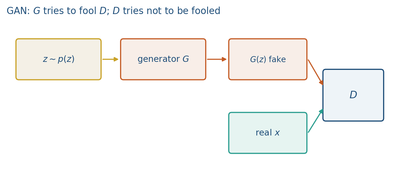
In this course is a tiny MLP (Lab 11: 8-D noise 2-D point). The same picture is a CNN or a transformer decoder when is an image or a spectrogram. The algebra does not change: sample , push it through , hand the fake to .
is ordinary supervised learning on a moving dataset: reals with label 1, fakes with label 0. The catch is that the fake distribution changes every time you update . You never have a fixed classification problem.
4. How it works, step by step
Training both nets, with the actual losses, is the next note. The idea you need today is what each player sees and what a Bayes-optimal would say.
- Draw noise and form a fake . does not compare that fake to the nearest real (that would be an autoencoder). The only teacher is ’s scalar.
- scores a mixed batch: reals from the data, fakes from the current .
- Update so reals go toward 1 and fakes toward 0, then update so goes toward 1. The min-max details live in note 11.2.
- Read the Bayes-optimal discriminator. Where matches the data, that optimum is a coin flip: . Where never goes, and . ’s loss never sees that missing location.
Suppose the reals are two spikes and an untrained always emits the right-hand spike. A Bayes-optimal is then on that spike (half real, half fake) and on the left spike (only reals). is “winning” at the right spike in the sense that . It is losing as a distribution: the left mode has zero fake mass. The worked example below puts numbers on that cartoon.
5. Mathematical formulas
The discriminator is a probability in :
The Bayes-optimal discriminator for a fixed generator (Goodfellow et al.) is
At a perfect , and everywhere the mass lives. That is success as a distribution, not a trophy for a single pretty fake. Where never goes, and .
6. Positive points and negative points
Positive.
- Sampling is one forward pass through , not a long reverse chain.
- When training holds, samples can be sharp rather than a blurry average of modes.
- The same two-player picture scales from Lab 11’s 2-D MLP to images and spectrograms without changing the algebra.
- You get an implicit generator when writing is the wrong tool.
Negative.
- There is no likelihood, no , and no test log-likelihood to report.
- Training is unstable (note 11.2): the classification problem moves every time updates.
- Mode collapse (note 11.3) is the usual coverage failure, not blur.
- This is not an LLM method. Do not mix it with next-token training.
When not to use a GAN. A task that needs a number for or an inference query . Diffusion (Week 12) if you would rather train a denoiser than fight an adversary, and you can afford iterative sampling.
7. Teaching this note
About 35 minutes at the board, then ~8 minutes of video. This is the first of three GAN notes in a two-hour class; Lab 11 uses the rest of the block.
- 0–12 min. Implicit vs explicit. You cannot write for a GAN. You can sample. Sketch the two-player diagram.
- 12–24 min. What and each see. never sees a real on its own update. never sees .
- 24–34 min. Worked 1-D two-mode example. Leave the numbers on the board; note 11.3 will reuse them.
- Then play 46:45–54:00 of the assigned video (GAN setup: give up on density, noise through a generator). Pause when the two-player cartoon appears.
8. Worked example
Reals are two spikes in 1-D: half the mass at , half at . (Lab 11 is the same idea in 2-D, means and .)
Suppose an untrained ignores and always emits .
A Bayes-optimal then scores:
| location | what sees | |
|---|---|---|
| half real, half fake | ||
| only reals | ||
| anywhere else | only fakes, if any | near |
is “winning” at in the sense that , a coin flip. It is losing as a distribution: the left mode has zero fake mass. One sample at looks perfect. The generator is not trained.
If you now let move and it jumps all mass to , the table flips: , . That oscillation is the seed of note 11.3.
The optimal discriminator is . Where never goes, and . ’s loss never sees that location.
9. Where students get stuck
- Treating one pretty fake as success. is a distribution, not a Photoshop filter.
- Thinking is trained by comparing to the nearest real (an autoencoder). It is not. The only teacher is ’s scalar.
- Forgetting that ’s data distribution moves. A that was perfect last step is scoring a different this step.
10. Video
Watch Generative models: GAN setup, 46:45–54:00.
Pause at the two-player setup: noise through a generator, no explicit density. Skip PixelCNN/VAE (the first 45 minutes) in class; those are not this note. Notes 11.2 and 11.3 reuse the same URL at later pause points.
11. Practice
-
never sees a real image on its own update (only through ’s scores). How can it learn the data distribution?
-
Why is a perfect (always 1 on reals, always 0 on fakes) a problem for ’s gradient?
-
Name one task where a GAN is a natural fit and one where an explicit likelihood model would be easier to evaluate.
-
In the 1-D example, always and reals are equal spikes at . What is the Bayes-optimal ? What is ?
-
You draw 10 fakes and all 10 equal . A classmate says “ is 0.5 there, so is done.” Write one sentence that disagrees, using coverage.