12.2 The Reverse Process

DATA 443/643 · Week 12 · PDF · Slides

MSE on the noise you added. T reverse steps. Lab 12 uses the oracle mean.

These notes match the lecture slides. Use (slides) on the course hub for the deck.

Generation walks the forward process backward. You start from ${\mathit{x}}_T~𝒩(\mathbf{0},𝐈)$ and, step by step, remove a bit of noise until you have ${\mathit{x}}_0$. By the end you should be able to write the noise-prediction loss, take one reverse-step mean, and say what Lab 12’s oracle is replacing.

1. What the diffusion reverse process is

The reverse is: predict the noise you added, take a step toward $x_0$, repeat $T$ times. A net ${\mathit{\epsilon }}_{\theta }({\mathit{x}}_t,t)$ predicts the $\mathit{\epsilon }$ from note 12.1. Training is ordinary MSE on that noise. Sampling starts from ${\mathit{x}}_T~𝒩(\mathbf{0},𝐈)$ and denoises.

Ho et al. (DDPM) made noise prediction the default parameterization. Predicting $\mathit{\epsilon }$ is equivalent (up to scaling) to predicting ${\mathit{x}}_0$ or the score ${\nabla }_{{\mathit{x}}_t}\log q({\mathit{x}}_t)$. Pick one parameterization and stay consistent.

You cannot write the true reverse kernel in closed form for images, because it would need the unknown data density. If you knew ${\mathit{x}}_0$, the true posterior $q({\mathit{x}}_{t-1}\mid {\mathit{x}}_t,{\mathit{x}}_0)$ is Gaussian with a closed-form mean. Lab 12 uses that oracle mean for a single step so you can see the geometry without training a U-Net. A trained ${\mathit{\epsilon }}_{\theta }$ is what replaces the known $\mathit{\epsilon }$ (and therefore the known $x_0$) at sample time.

2. Why we use it

MSE on a known $\mathit{\epsilon }$ is easier than a GAN min-max. There is no discriminator to race. The forward jump from note 12.1 already gave you ${\mathit{x}}_t$ in one line, so the loss never unrolls a reverse chain.

The cost sits at sample time. You pay $T$ network calls (or fewer with DDIM / distilled samplers). That is the trade: stable regression training, slow ancestral sampling. GANs (Week 11) sample in one forward pass and fight mode collapse instead.

For a project, report the sampler ($T$, DDPM vs DDIM) next to the metric. Changing $T$ at test time is part of the method. Classifier-free guidance, which steers the same reverse chain with a text condition, is the next note.

3. Architecture

The network is a denoiser that sees a noisy input and a timestep: a U-Net or a DiT on ${\mathit{x}}_t$ with a time embedding. The same ${\mathit{x}}_t$ is a different problem at $t=10$ and at $t=900$, so $t$ is an input, not a footnote.

Lab 12 uses an oracle mean so you see the geometry without training. You are not training a U-Net in that lab. You know ${\mathit{x}}_0$, so you can form the true posterior mean and check that one reverse step moved closer.

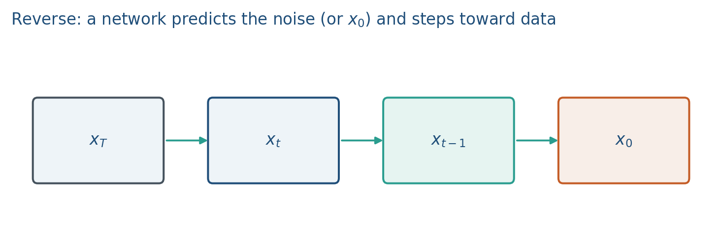
Sampling is an iterative procedure. Start at ${\mathit{x}}_T$, apply the reverse-step mean (plus a little noise except at $t=1$), and walk down to ${\mathit{x}}_0$. Each step is one network call once ${\mathit{\epsilon }}_{\theta }$ exists.

4. How it works, step by step

Training is ordinary regression.

1. Sample ${\mathit{x}}_0$ from the data, $t$ uniformly from $1\dots T$, and $\mathit{\epsilon }~𝒩(\mathbf{0},𝐈)$.
2. Form ${\mathit{x}}_t$ with the one-liner from note 12.1.
3. Predict ${\mathit{\epsilon }}_{\theta }({\mathit{x}}_t,t)$. Take MSE against the true $\mathit{\epsilon }$. No adversary. No reverse chain inside the loss.

Sampling is the reverse walk.

1. Draw ${\mathit{x}}_T~𝒩(\mathbf{0},𝐈)$.
2. For $t=T,\dots ,1$, plug ${\mathit{\epsilon }}_{\theta }({\mathit{x}}_t,t)$ into the reverse-step mean below, and add ${\sigma }_t\mathit{z}$ for $t>1$.
3. Return ${\mathit{x}}_0$.

If you knew ${\mathit{x}}_0$, Lab 12 skips the net and uses the true posterior mean for a single step. The lab check is $\Vert x_t-x_0\Vert$ versus $\Vert \widehat{x}-x_0\Vert$ at $t=20$: the second should be smaller. If ${\epsilon }_{\theta }=0$ (the net refuses to denoise), the subtracted term vanishes and you mostly rescale $x_t$, which is not a sample from the data.

5. Mathematical formulas

The training loss is

Given ${\mathit{x}}_t$ and a noise prediction, a typical mean for ${\mathit{x}}_{t-1}$ is

with $\mathit{z}~𝒩(\mathbf{0},𝐈)$ for $t>1$, and ${\sigma }_t$ from the schedule (often ${\sigma }_t^2={\beta }_t$). At a generic $t$ you do not jump all the way to ${\mathit{x}}_0$; you move closer. Forgetting ${\sigma }_{t}z$ on the way down makes every sample look identical.

6. Positive points and negative points

Positive.

• MSE on $\epsilon$ is ordinary regression, which is easier to stabilize than a GAN min-max.
• Predicting $\epsilon$ is enough: it is equivalent (under the usual parameterization) to predicting the posterior mean.
• Lab 12’s oracle mean lets you see one reverse step without training a U-Net.
• You can change $T$ (or switch to DDIM) at sample time and treat the sampler as part of the method.

Negative.

• Ancestral sampling costs many network calls; quality versus speed is a real knob.
• Omitting $t$ as an input makes the same $x_t$ look like one problem at every noise level.
• Dropping ${\sigma }_{t}z$ collapses diversity: every run hugs the mean.
• Classifier-free guidance, which steers this chain with text, is extra machinery (next note).

When not to. If you need one-pass samples and can live with collapse, that is still a GAN. If you need text control, do not stop at this unconditional reverse chain.

7. Teaching this note

About 35 minutes at the board, then ~6 minutes of video.

• 0–10 min. MSE on $\epsilon$. Same $x_t$ formula as 12.1.
• 10–22 min. Write one reverse-step mean. Circle the ${\epsilon }_{\theta }$ term.
• 22–33 min. Worked scalar reverse step, then the Lab 12 oracle story.
• Then play Umar Jamil 13:00–16:36 (training loop, then sampling loop). Pause when he draws one denoising step.

8. Worked example

Reuse $x_0=1.0$, ${\overline{\alpha }}_t=0.64$, $\epsilon =2.0$, so $x_t=2.0$ as in note 12.1. Take ${\alpha }_t=0.64$ for a single-step cartoon (so $\sqrt{{\alpha }_t}=0.8$, $1-{\alpha }_t=0.36$, $\sqrt{1-{\overline{\alpha }}_t}=0.6$).

Suppose ${\epsilon }_{\theta }=\epsilon =2.0$ exactly, and drop ${\sigma }_{t}z$ for the mean:

The reverse mean lands on $x_0$. That is the oracle: if you predict the true noise, one algebraic step peels it off (here ${\alpha }_t={\overline{\alpha }}_t$, a first-step special case). At a generic $t$ you do not jump all the way to $x_0$; you move closer. Lab 12 checks $\Vert x_t-x_0\Vert$ vs $\Vert \widehat{x}-x_0\Vert$ at $t=20$ and wants the second smaller.

If ${\epsilon }_{\theta }=0$ (the net refuses to denoise), the subtracted term vanishes and you mostly rescale $x_t$, which is not a sample from the data.

2.0 peels back to $1.0$" src="files/graphics/12.2-diffusion-reverse/reverse-mean.png" />

Sampling is an iterative procedure. You pay $T$ network calls (or fewer with DDIM). A GAN still samples in one pass and fights collapse instead.

9. Where students get stuck

• Training a U-Net in Lab 12. The lab uses the true posterior mean because you know $x_0$.
• Omitting $t$ as an input to ${\epsilon }_{\theta }$. The same $x_t$ is a different problem at $t=10$ and at $t=900$.
• Forgetting ${\sigma }_{t}z$ on the way down and then wondering why every sample looks identical.

10. Video

Watch Umar Jamil, How diffusion models work, 13:00–16:36.

Pause on the training objective (predict the noise) and on the sampling loop (many reverse steps). Same URL as note 12.1; do not replay 7:35–13:00 unless needed.

11. Practice

1. If ${\mathit{\epsilon }}_{\theta }=\mathit{\epsilon }$ exactly, what should happen to $\Vert {\mathit{x}}_{t-1}-{\mathit{x}}_0\Vert$ relative to $\Vert {\mathit{x}}_t-{\mathit{x}}_0\Vert$, in expectation, for mid-range $t$?

2. Why add ${\sigma }_t\mathit{z}$ on the way down instead of always taking the mean?

3. You may not train a score network in Lab 12. What replaces ${\mathit{\epsilon }}_{\theta }$ for that one reverse step?

4. $x_t=3$, ${\alpha }_t=0.25$, ${\overline{\alpha }}_t=0.25$, ${\epsilon }_{\theta }=2$, no extra noise. Compute the reverse mean. ($\sqrt{{\alpha }_t}=0.5$, $\sqrt{1-{\overline{\alpha }}_t}=\sqrt{0.75}\approx 0.866$, $1-{\alpha }_t=0.75$.)

5. Training samples $t$ uniformly from $1\dots T$ and one $\epsilon$. Why is that enough, instead of a full reverse chain inside the loss?