12.1 The Forward Process

DATA 443/643 · Week 12 · PDF · Slides

Jump to x_t in one shot. α-bar from 1 to 0. The kernel is not learned.

These notes match the lecture slides. Use (slides) on the course hub for the deck.

A diffusion model learns to denoise. The forward process is not learned. You add Gaussian noise on a schedule until the sample is almost prior noise. Training later asks a net to predict that noise. By the end you should be able to write ${\alpha }_t$ and ${\overline{\alpha }}_t$, jump to any $t$ in one line, and say why that jump is nicer to train than a GAN min-max.

1. What the diffusion forward process is

Diffusion (DDPM) destroys a sample with Gaussian noise on a schedule, then later learns to reverse it. Start from data ${\mathit{x}}_0$. A variance schedule $0<{\beta }_t<1$ (small at first, larger later) defines a Markov chain ${\mathit{x}}_0\to {\mathit{x}}_1\to \cdots \to {\mathit{x}}_T$. At $t=0$ you still have the data. At $t=T$ you have nearly isotropic noise.

The forward kernel is fixed. There is no $\theta$ in $q$. You do not have to simulate every hop. The marginal $q({\mathit{x}}_t\mid {\mathit{x}}_0)$ is a closed-form Gaussian that interpolates from data to noise, so you can jump to any $t$ in one shot.

In code that jump is one line: sample $\mathit{\epsilon }~𝒩(\mathbf{0},𝐈)$ and mix it with ${\mathit{x}}_0$ using ${\overline{\alpha }}_t$. Training (note 12.2) samples a random $t$, draws $\mathit{\epsilon }$, forms ${\mathit{x}}_t$ in one shot, and asks a net to guess $\mathit{\epsilon }$. You never need to walk $1,2,\dots ,t$ unless you want a picture of the path.

2. Why we use it

GANs fight a min-max. Diffusion trains a denoiser with MSE. The kernel is not learned, so there is no discriminator to race. The training signal at each $t$ is a denoising regression against a known $\mathit{\epsilon }$.

Coverage is not automatic, but you are not playing an adversarial game. That is the trade this week is for. You still have to pick $\{{\beta }_t\}$ and $T$. Sampling will be a reverse chain (note 12.2), which is slower than one GAN forward pass.

Likelihood-related bounds exist for this family in a way they do not for a vanilla GAN. You do not need the ELBO on the board today. You need: the forward process is a fixed noising schedule, and that is why the loss can be ordinary regression.

3. Architecture

The architecture of this note is a Markov chain, not a U-Net. (The net arrives in note 12.2.) A variance schedule ${\beta }_t$ or, equivalently, ${\overline{\alpha }}_t$ falling from near 1 to near 0, defines

The Markov step is $q({\mathit{x}}_t\mid {\mathit{x}}_{t-1})=𝒩({\mathit{x}}_t;\sqrt{{\alpha }_t}{\mathit{x}}_{t-1},{\beta }_t𝐈)$. The marginal is closed form, so training never has to unroll the chain.

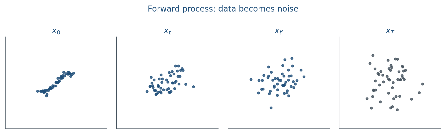
${\overline{\alpha }}_t$ starts near 1 (the point is still itself) and falls toward 0 (the point is almost $\mathit{\epsilon }$). Linear, cosine, and learned ${\beta }_t$ are all ways to spend more steps where structure dies. Too fast a schedule and early $t$ is already junk; too slow and you waste capacity on near-copies of ${\mathit{x}}_0$.

$T$ (often 1000 in image papers) is a discretization. Lab 12 uses a small $T$ in 2-D so you can plot the path. Print ${\overline{\alpha }}_1$, ${\overline{\alpha }}_{T/2}$, ${\overline{\alpha }}_T$: they should fall.

4. How it works, step by step

The whole point of this note is that you can skip the chain at train time.

1. Choose a schedule $\{{\beta }_t\}$ and precompute ${\alpha }_t=1-{\beta }_t$ and ${\overline{\alpha }}_t={\prod }_{s=1}^t{\alpha }_s$.
2. Take a clean sample ${\mathit{x}}_0$ (Lab 12: a 2-D point).
3. Draw a timestep $t$ (training will draw it at random) and a noise $\mathit{\epsilon }~𝒩(\mathbf{0},𝐈)$.
4. Form ${\mathit{x}}_t=\sqrt{{\overline{\alpha }}_t}{\mathit{x}}_0+\sqrt{1-{\overline{\alpha }}_t}\mathit{\epsilon }$ in one shot. Do not loop $s=1,\dots ,t$.
5. Hold ${\mathit{x}}_t$ and $\mathit{\epsilon }$ for the reverse note: the net will be asked to guess $\mathit{\epsilon }$.

If ${\overline{\alpha }}_t=1$, then ${\mathit{x}}_t={\mathit{x}}_0$. If ${\overline{\alpha }}_t=0$, then ${\mathit{x}}_t=\mathit{\epsilon }$. Mid-range ${\overline{\alpha }}_t$ is a mix: more noise than signal once ${\overline{\alpha }}_t$ is no longer close to 1. Same arithmetic in Lab 12 with a vector $x_0=(1.5,-0.8)$ and a vector $\epsilon$. The square roots are scalar; they multiply every coordinate.

5. Mathematical formulas

The one-step kernel and the closed-form marginal are

The reparameterization you type in code is

That one-liner is why the loss never walks $1,\dots ,t$.

6. Positive points and negative points

Positive.

• The forward kernel is fixed, so the training target is a known $\mathit{\epsilon }$ rather than a moving adversary.
• You can jump to any $t$ with one Gaussian draw, which makes training a single MSE later.
• The schedule is inspectable: print ${\overline{\alpha }}_1$, ${\overline{\alpha }}_{T/2}$, ${\overline{\alpha }}_T$ and watch them fall.
• The same algebra runs in Lab 12’s 2-D points and in image DDPMs.

Negative.

• The forward process is the easy half. Reverse sampling (note 12.2) is slow: you pay many network calls.
• A too-fast $\{{\beta }_t\}$ crashes ${\overline{\alpha }}_t$ in a few steps and the net never sees a lightly noised ${\mathit{x}}_0$.
• A too-slow schedule wastes capacity on near-copies of the data.
• This is not a GAN: you gave up one-pass sampling in exchange for a stable regression.

When not to. If you need a sample in one forward pass and you can live with coverage bugs, that is still a GAN (Week 11).

7. Teaching this note

About 35 minutes at the board, then ~6 minutes of video. First of three Week-12 notes.

• 0–12 min. Markov step vs closed-form marginal. Write ${\alpha }_t$ and ${\overline{\alpha }}_t$.
• 12–22 min. The one-line reparameterization. Draw $x_0$ mixing with $\epsilon$.
• 22–33 min. Worked scalar step. Change ${\overline{\alpha }}_t$ from 1 to 0 and watch $x_t$.
• Then play Umar Jamil 7:35–13:00 (forward/reverse cartoon, then the math of $q$). Pause on the closed-form $q(x_t\mid x_0)$.

8. Worked example

Take a 1-D point $x_0=1.0$ and a draw $\epsilon =2.0$. Then

At ${\overline{\alpha }}_t=0.64$ you already sit at $2.0$: more noise than signal. At ${\overline{\alpha }}_t=0$ you have thrown $x_0$ away; $x_t$ is just $\epsilon$.

Same arithmetic in Lab 12 with a vector $x_0=(1.5,-0.8)$ and a vector $\epsilon$. The square roots are scalar; they multiply every coordinate.

You can jump to any $t$ without simulating $q(x_s\mid x_{s-1})$ for $s=1,\dots ,t$. That is why training is a single Gaussian draw, not a loop of length $t$.

α¯t values on $x_0=1$, $\epsilon =2$" src="files/graphics/12.1-diffusion-forward/alphabar.png" />

Pick a noise level, corrupt $x$, then learn to undo a bit. The closed-form jump is why the loss never walks $1,\dots ,t$.

9. Where students get stuck

• Simulating all $T$ Markov steps at train time. You sample $t$ and use $q(x_t\mid x_0)$.
• Mixing up ${\beta }_t$, ${\alpha }_t$, and ${\overline{\alpha }}_t$. Write the three definitions every time.
• Setting every ${\beta }_t$ huge. Then ${\overline{\alpha }}_t$ crashes in a few steps and the net never sees a lightly noised $x_0$.

10. Video

Watch Umar Jamil, How diffusion models work, 7:35–13:00.

Pause on the forward process $q$ (no $\theta$) and the closed-form jump to $x_t$. Skip the U-Net coding (after ~16:30) in this class. Note 12.2 continues the same video at the training/sampling chapters.

11. Practice

1. If ${\overline{\alpha }}_t=1$, what is ${\mathit{x}}_t$? If ${\overline{\alpha }}_t=0$, what is ${\mathit{x}}_t$?

2. Why can you sample ${\mathit{x}}_t$ in one line instead of looping $t$ steps of $q({\mathit{x}}_s\mid {\mathit{x}}_{s-1})$?

3. A classmate sets every ${\beta }_t=0.9$. What goes wrong in the first few $t$?

4. $x_0=4$, ${\overline{\alpha }}_t=0.25$, $\epsilon =-1$. Compute $x_t$. ($\sqrt{0.25}=0.5$, $\sqrt{0.75}\approx 0.866$.)

5. ${\beta }_1=0.1$, ${\beta }_2=0.2$. Compute ${\alpha }_1,{\alpha }_2,{\overline{\alpha }}_2$.