
3.1 From Recurrence to Attention
The seq2seq bottleneck, then a path of length one at cost T squared.
These notes match the lecture slides. Use (slides) on the course hub for the deck.
An RNN compresses the whole past into one vector, so token 1 can affect token 40 only by surviving 39 overwrites. Attention lets every token look at every other token in one step: that is the move from Week 2’s recurrences to the rest of the course. By the end you should be able to contrast path length with cost , and say where Bahdanau’s queries come from versus self-attention.
1. What attention is
Attention is a path of length one between any two positions. Instead of squeezing a sentence into one RNN hidden state, each output position looks at all encoder states with a weighted sum.
A seq2seq RNN encodes the source into one vector, then the decoder must generate from that vector. Long source, same-size bottle. Attention is a direct connection from the decoder to the encoder states, so the model can reread instead of remember.
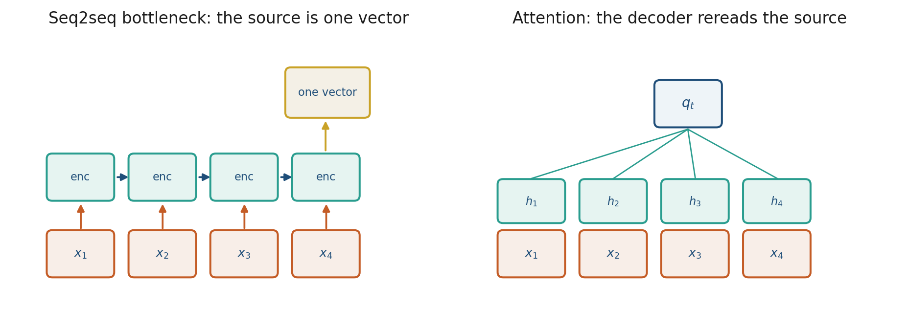
Bahdanau et al. (2015) added that reread on top of an RNN. Queries come from the decoder; keys and values come from the encoder. Vaswani et al. (2017) dropped the recurrence: self-attention is the layer, and every token in the same sequence plays all three roles.
Draw The cat … it with 40 dots. RNN: 39 arrows in a line. Attention: one arrow from it to cat, plus arrows to everyone else, with weights. Note 3.2 turns those weights into softmax.
2. Why we use it
Seq2seq RNNs have a bottleneck: one vector for the whole source. Long sources forget the beginning. Week 2’s Jacobian product is the learning-story version of the same complaint: token 1 reaches token only through multiplies.
The path-length win is why that product stops being the story. Parallel over time is why pretraining scaled: given all embeddings , you form with matrix multiplies a GPU likes. An LSTM must finish step before step . That, more than “transformers are magic,” is why this week exists.
If each RNN Jacobian factor is , the product over 39 steps is . Attention’s hop is . That is Week 2 meeting Week 3.
3. Architecture
Encoder states . Decoder query . Weights over the source, then a mix. Self-attention (next note) uses the same sequence for query and keys.
| RNN | Self-attention | |
|---|---|---|
| Path length, token 1 to | ||
| Parallel over time | no | yes |
| Cost in | memory/time for full attention |
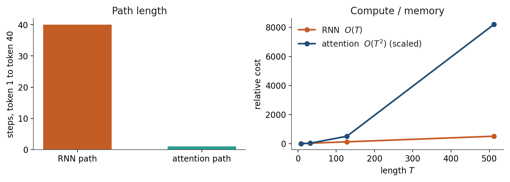
Path length 1 is not cost 1. The bill is why Week 7 exists. For this course’s default, full attention is the model.
Write and for . Sparse or sliding-window attention is what you do when no longer fits. You still teach full attention first.
FlashAttention changes the implementation, not the fact that every pair can interact. Decoder-only GPT still pays in training. At decode time, caching keys and values makes each new token against the past. That is inference, not the training flop count.
Keep the slogan: RNN path , attention path , attention cost .
4. How it works, step by step
Score, softmax, weighted sum. Cost is scores, not path length . The formula lives in note 3.2; this note is why you bother.
Take a sentence of length : cat, sat, on, it.
- An RNN path from
cattoitis 3 sequential steps. Each step overwrites a hidden state. - Attention writes one score in the last row of a matrix:
itlooking atcat, and also at everyone else. - Full attention stores scores. Four tokens’ queries can be dotted with keys in one matmul. An LSTM needs four sequential cell calls.
- Scale that picture to a 4k-token PDF: , scores per head per layer. If one score is 4 bytes, that is about MB for one map, before batching and before stacking layers. That is the quadratic complaint.
Bahdanau’s additive score is one way to get the weights (formula in section 5). Scaled dot-product self-attention is the default from here on.
5. Mathematical formulas
Path length 1 at cost for a sequence of length and width .
Bahdanau’s additive score for decoder query against encoder state :
The attention weights are a softmax of those scores, then a weighted sum of the values (encoder states, for Bahdanau). Note 3.2 replaces this with scaled dots .
RNN versus attention, in one line: path length from token 1 to is versus ; flop count in is versus .
6. Positive points and negative points
Positive.
- No sequential bottleneck: any two positions interact in one hop, so Week 2’s Jacobian product is no longer the long-range story.
- The mix is a weighted sum you can plot; large mass on a name is a readable “this pronoun looked at that name.”
- Given all embeddings, are matrix multiplies a GPU likes, so you can batch a whole sentence’s updates at once.
- Caching keys and values at decode time makes each new token against the past (inference, not training).
Negative.
- Quadratic cost in : memory and time for a full attention map grow as .
- Path length 1 is not compute. Hearing “one hop” and writing is the usual slip.
- Bahdanau attention still sits on an RNN; it is not yet “attention instead of recurrence.”
- KV cache does not change the training cost of a full attention map.
When not to. For tiny , an RNN’s loop can be enough and cheaper. When no longer fits, you change the pattern (sparse or sliding window) after you understand full attention.
7. Teaching this note
~16 minutes. Bottleneck picture, Bahdanau vs self-attention in one sentence, then the path-length table and the vs arithmetic. Play 0:00–12:00 of 3Blue1Brown’s GPT visual intro (next-token prediction and the first all-to-all cartoon). Do not derive QKV here; that is note 3.2.
8. Worked example
Sentence length tokens: cat, sat, on, it.
RNN path from cat to it: 3 steps. Attention path: 1 score in the last row of a matrix.
Full attention stores scores. For a 4k-token PDF, , scores per head per layer. If one score is 4 bytes, that is about MB for one map, before batching and before stacking layers. That is the quadratic complaint.
GPU parallel: four tokens’ queries can be dotted with keys in one matmul. LSTM: four sequential cell calls.
If each RNN Jacobian factor is , the product over 39 steps is . Attention’s hop is . That is Week 2 meeting Week 3.
9. Where students get stuck
- Hearing “path length 1” and thinking attention is compute (it is ).
- Mixing Bahdanau (attention on an RNN) with Vaswani (attention instead of an RNN).
- Believing the RNN state “contains the whole sentence” in a lossless way.
10. Video
Watch 3Blue1Brown: But what is a GPT? Visual intro to transformers.
Pause when next-token prediction is a stack of vectors, and at the first all-to-all attention cartoon. Stop before the full QKV derivation if you are teaching 3.2 next.
11. Practice
-
Why can a transformer GPU-batch a whole sentence’s updates at once, while an LSTM cannot?
-
A 4k-token policy PDF: what is the quadratic cost complaining about?
-
In one sentence, what information did have to store that an attention row can fetch instead?
-
For , how many attention scores are in one head’s map? For , how many? What is the ratio ?
-
An RNN of length has path length from token 1 to token 50. Write the attention path length. If each RNN Jacobian factor is , bound the RNN product vs attention’s single hop of .
-
Bahdanau versus Vaswani, in one sentence each: where do the queries come from?
-
Caching keys and values at decode time makes each new token cheaper. Does that change the training cost of a full attention map? Why or why not?