6.2 Traditional Text Classification

BoW or TF-IDF features with a linear or neighbor model.

These notes walk through the lecture slides. The original deck is unchanged; use (slides) on the course hub if you want that PDF.

1. Two classical classifiers

Once the document is a vector (BoW or TF–IDF from Week 4), you can use any supervised model. Lecture walks two that you should be able to explain: $k$ -nearest neighbors and a linear SVM.

The rest of the note is how you choose hyperparameters and how you score the classifier when classes are not 50/50. That part matters more than the algebra.

Practical Natural Language Processing is the course text. The pictures of CV and metrics are standard ML.

2. $k$ -nearest neighbors

Store the training set. To label a new point, find the $k$ nearest training vectors (Euclidean or cosine) and take a majority vote.

k-NN in the plane

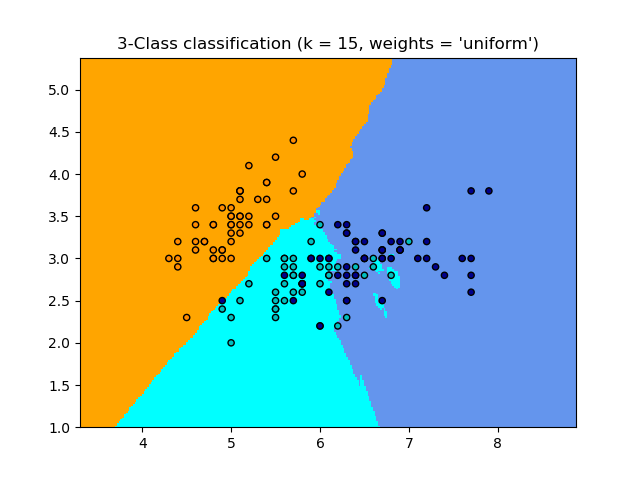
There are no weights to learn. The whole training matrix is the model. That is fine for a few thousand short documents and painful for a million.

$k$ is a hyperparameter. Small $k$ follows local noise. Large $k$ smooths toward the majority class. On TF–IDF, cosine is the usual distance.

3. Linear SVM

Training pairs $(𝐱_{i}, y_{i})$ with $y_{i} \in {+ 1, - 1}$ . A linear SVM finds a hyperplane $𝐰 \cdot 𝐱 - b = 0$ that separates the classes with the largest margin.

You minimize $‖ 𝐰 ‖$ subject to $y_{i} (𝐰 \cdot 𝐱_{i} - b) \geq 1$ .

Maximum-margin separator

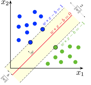
In text, $𝐱$ is usually L2-normalized TF–IDF. LinearSVC or SGDClassifier(loss="hinge") is what you call. A kernel SVM on a 50,000-column bag is rarely worth it. The linear version is the baseline to beat.

4. Cross-validation and hyperparameters

Parameters are what the learner sets from data: $𝐰$ , the support vectors, the neighbor labels. Hyperparameters are what you set: $k$ , the SVM’s $C$ , max_features, n-gram range. If you tune $C$ on the same fold you report, the score is optimistic.

Hold-out: train / validation / test. Fit on train, pick hyperparameters on validation, report once on test.

$K$ -fold: split train into $K$ pieces. Each piece is validation once. Average the $K$ scores. Use this when the data set is not huge.

Nested CV: the inner loop picks hyperparameters; the outer loop estimates generalization. That is the honest number when you need one number for a paper or a client and you already used the data to search.

If you only remember one rule: the test set is not a tuning knob.

5. Metrics when accuracy lies

Accuracy is correct / total. It is fine when classes are balanced. It is not fine when 95% of tickets are “general inquiry.” A model that always says “general” is 95% accurate and useless.

For a class you care about (say happy):

Metric	Question it answers
Precision	Of the docs I called happy, how many were?
Recall	Of the happy docs, how many did I find?
F1	Harmonic mean of the two
ROC	True-positive rate vs false-positive rate as you move the threshold

Precision and recall

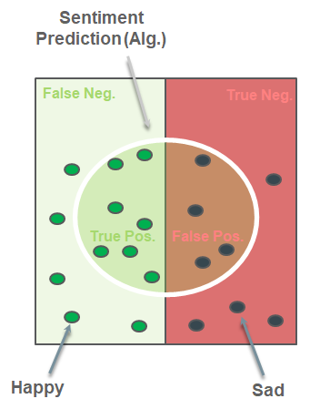
F1 punishes a system that only wins on one of the two. ROC / AUC is useful when you will pick a threshold later.

sklearn: precision_score, recall_score, f1_score, roc_curve, and classification_report.

from sklearn.metrics import classification_report
print(classification_report(y_true, y_pred, target_names=["class 0", "class 1", "class 2"]))

Read the per-class rows, not just the headline accuracy.

6. Practice

Training data are 90% ham. A filter that never flags spam has high accuracy. Which metric exposes that it found no spam?
You pick $k$ by maximizing accuracy on the test set. What is wrong, and what should you use instead?
Why is a linear SVM the usual text baseline rather than an RBF kernel SVM?

Ahmad Mousavi