13.2 SVD and Topic Modeling

Latent semantic analysis from a word-document matrix.

These notes walk through the lecture slides. The original deck is unchanged; use (slides) on the course hub if you want that PDF.

1. Topics from a decomposition

Bag-of-words and TF–IDF give you a matrix. If you factor that matrix, the factors are often readable as topics.

That idea is latent semantic analysis (LSA): treat the DTM as $A$ and take a low-rank SVD.

Topics as latent structure

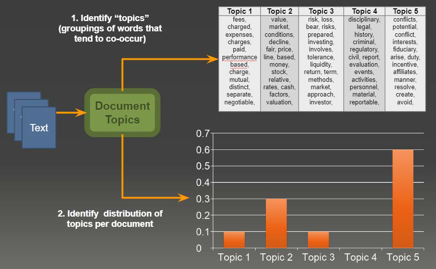
A topic here is not a human essay title. It is a group of terms that travel together (classroom, teacher, student → a "school" factor) plus a weight for how much each document uses that group.

2. SVD, truncated

Any real matrix has a singular value decomposition. For topic modeling we keep the top $r$ components:

A \approx U_{r} Σ_{r} V_{r}^{*} .

Truncated SVD

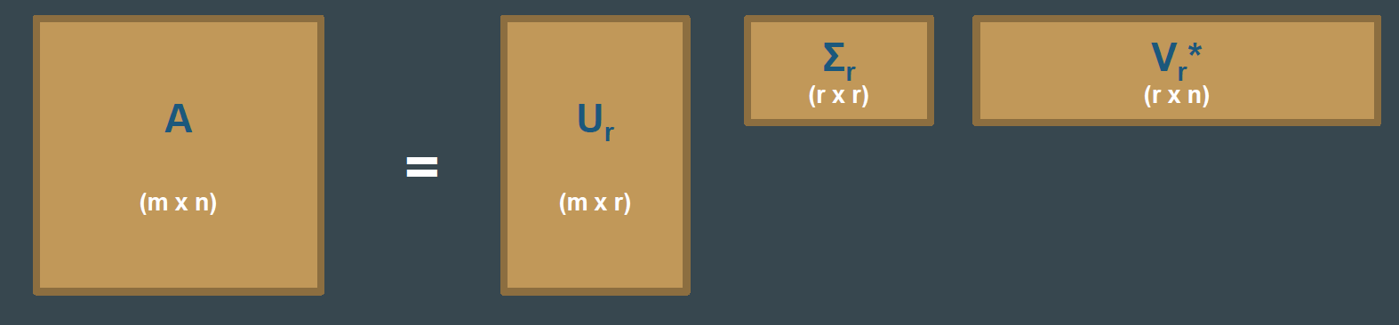
Factor	Shape	Reading
$A$	$m \times n$	Terms × documents (or the transpose; be consistent)
$U_{r}$	$m \times r$	How each term loads on each of $r$ topics
$Σ_{r}$	$r \times r$	Diagonal. Size of each topic (importance)
$V_{r}^{*}$	$r \times n$	How each document mixes those topics

$U_{r}$ is the dictionary: topic 1 is the terms with large entries in column 1. $Σ_{r}$ ranks the topics. $V_{r}^{*}$ is the recipe for each document (30% topic 1, 50% topic 2, …).

The number $r$ is a choice. Too small and you merge distinct themes. Too large and you split noise into fake topics.

3. SVD and PCA are cousins

PCA on centered data is SVD on the covariance, or SVD on the data matrix itself.

Left singular vectors of $A$ live in $U$ .
Singular values $σ_{i}$ sit on the diagonal of $Σ$ .
For centered data, $σ_{i} = \sqrt{λ_{i}}$ where $λ_{i}$ is an eigenvalue of the covariance.

If you already centered the DTM and ran PCA, you have done a form of LSA. SVD is the cleaner statement when the matrix is rectangular (terms × documents), which a covariance matrix is not.

4. Why people still run it

Helps. Dimensionality drops: a huge TF–IDF matrix becomes $r$ factors. Noise in the small singular values is thrown away. Topics are linear combinations of terms, so you can read the top words. The algorithm is old, stable, and in every scientific stack.

Hurts.

Limitation	What it means on text
Terms treated as independent	Collocations and polarity can be split or mashed
Global only	No sentence window; bank is one column
Cost on sparse data	A wide DTM is expensive to factor in one shot
Needs the full matrix	Awkward for a stream of new documents
Negative entries	A term can load negatively on a topic; hard to explain to a client
No built-in $r$	You try several ranks and look at the words

LSA is a strong baseline. Week 14 adds LDA (generative, non-negative mixtures) and NMF (additive, non-negative factors). Those exist in part to fix the last two rows.

When you run it, inspect the top terms in each column of $U_{r}$ , not only the reconstruction error. A small error with unreadable factors is a failed topic model. A slightly worse error with namable columns is a success.

sklearn's TruncatedSVD on a TF–IDF matrix is the usual first run. Try $r \in {10, 20, 50}$ , print ten terms per component, and stop when new components are noise. That is LSA in practice.

5. Practice

In one sentence each, what do $U_{r}$ , $Σ_{r}$ , and $V_{r}^{*}$ mean for a news corpus?
A topic has large positive weight on goal and large negative weight on election. Why is that awkward to show a reader, and which later method avoids the sign?
You add 500 documents every night. Why is a one-shot SVD a poor production fit?

Nightly full SVD is a batch job. If that job cannot finish before morning, you need an incremental method or a periodic re-fit, not a larger $r$ .

Folding in a new document with $U_{r}$ is an approximation. Recompute when the vocabulary or the mix of themes has moved.

Ahmad Mousavi

1. Topics from a decomposition

2. SVD, truncated

3. SVD and PCA are cousins

4. Why people still run it

5. Practice