
5.1 Introduction to Deep Learning
Layers, loss, and why we stack representations.
These notes walk through the lecture slides. The original deck is unchanged; use (slides) on the course hub if you want that PDF.
1. Why this note is here
Week 4 gave you sparse vectors. The rest of the course feeds those (or denser ones) to neural nets. This note is a first look at a net, not a survey of NLP architectures.
Figures and the MNIST walk-through follow Chollet, Deep Learning with Python (2nd ed.), and Géron, Hands-On Machine Learning.
2. A short history
McCulloch and Pitts (1943) wrote a logical model of how neurons might compute. That is the start of artificial neural networks (ANNs).
Interest came back in the 1980s (connectionism, better architectures, better training) and then faded. In the 1990s, support vector machines looked cleaner and worked well. Networks spent another winter.
Three things ended that winter:
- Data. Large labeled sets exist now. On those sets, nets often beat the older methods.
- Compute. GPUs, built for games, make the matrix multiplies cheap enough to train deep stacks.
- Algorithms. Better initializations, activations, and optimizers. Funding followed headlines; headlines followed products.
Hinton, Bengio, and LeCun shared the 2018 Turing Award for that line of work.
You do not need the history on an exam. You do need the reason we switched: when the representation is learned in layers, and you have enough data, the older sparse recipes lose.
3. A first network: MNIST
The job: 28 28 grayscale handwritten digits, ten classes (0–9).

Keras gives you the split already labeled:
from tensorflow.keras.datasets import mnist
(train_images, train_labels), (test_images, test_labels) = mnist.load_data()
# train_images.shape -> (60000, 28, 28)
# test_images.shape  -> (10000, 28, 28)
Sixty thousand training images, ten thousand held out. Labels are integers 0–9.
4. Layers, compile, fit
A layer is a transformation. Stack layers and you have a network. Each layer keeps what helps the task.
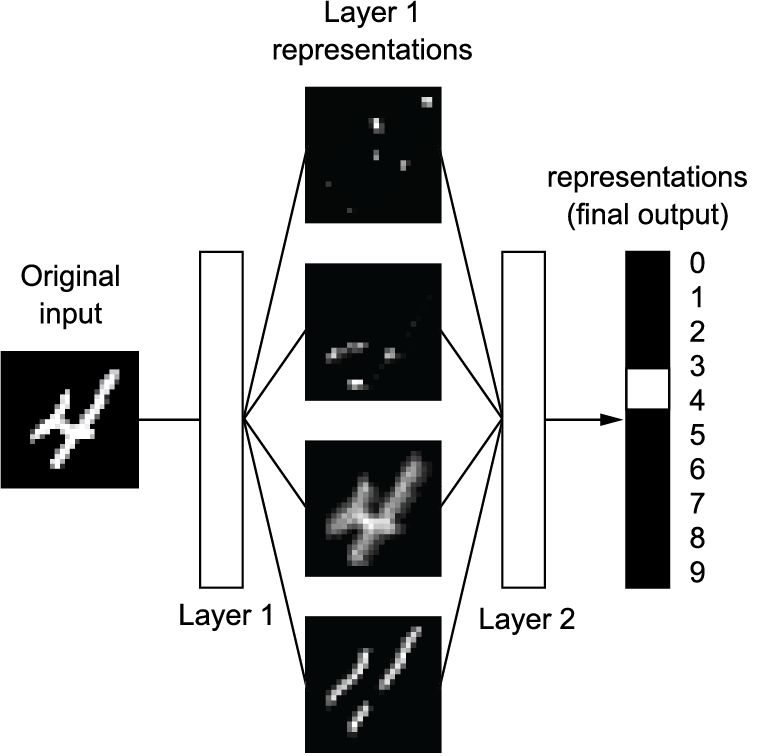
A two-layer classifier for MNIST:
from tensorflow import keras
from tensorflow.keras import layers
model = keras.Sequential([
    layers.Dense(512, activation="relu"),
    layers.Dense(10, activation="softmax"),
])
The last layer is a 10-way softmax: ten numbers that sum to 1, read as class probabilities.
Compile picks three things:
| Piece | Role |
|---|---|
| Optimizer | How weights move after each batch (rmsprop, adam, …) |
| Loss | How wrong the current answer is (sparse_categorical_crossentropy for integer labels) |
| Metric | What you watch (accuracy) |
model.compile(optimizer="rmsprop",
              loss="sparse_categorical_crossentropy",
              metrics=["accuracy"])
Pixels arrive as uint8 in . Flatten and scale to :
train_images = train_images.reshape((60000, 28 * 28)).astype("float32") / 255
test_images  = test_images.reshape((10000, 28 * 28)).astype("float32") / 255
Fit needs a batch size (how many examples before a weight update) and epochs (full passes through the training set):
model.fit(train_images, train_labels, epochs=5, batch_size=128)
The console prints training loss and training accuracy. Those are not the test numbers.
5. Predict and evaluate
predictions = model.predict(test_images[:10])
predictions[0].argmax()          # predicted digit
test_loss, test_acc = model.evaluate(test_images, test_labels)
argmax on a softmax row is the predicted class. Always report test accuracy. Training accuracy can look fine while the net memorizes.
3Blue1Brown’s neural-net videos are a useful watch after this note. They are not a substitute for running the cells.
Week 5 then leaves pixels and asks how to learn word vectors the same way: a small net, a prediction task, and the hidden weights kept as the representation.
6. Practice
-
Why do we divide pixel values by 255 before
fit? -
What does the softmax layer output, and why must those ten numbers sum to 1?
-
You see 99% training accuracy and 70% test accuracy after 20 epochs. What is the model doing, and which of the two numbers do you quote?