7.1 tidyr: Tidy Data and pivot_longer()

DATA 412/612 · Week 7 · PDF · Source (.qmd)

One variable per column, one observation per row. pivot_longer() turns wide columns into rows, and can strip a prefix, set a type, and drop missing cells.

1. Tidy data

A table is tidy when:

each variable is a column
each observation is a row
each value is a cell

That is a shape, not a quality judgment. A tidy table can still have missing values, typos, and bad types. A clean table has those problems handled. You usually tidy first, then clean.

tidyr is the tidyverse package for the shape. It loads with library(tidyverse).

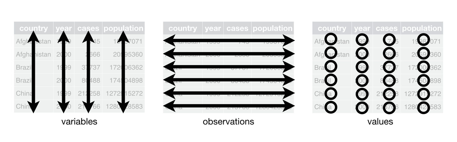
library(tidyverse)

2. `table1` is tidy; `table4a` is not

tidyr ships small WHO tuberculosis tables. ?table1.

table1

## # A tibble: 6 × 4
##   country      year  cases population
##   <chr>       <dbl>  <dbl>      <dbl>
## 1 Afghanistan  1999    745   19987071
## 2 Afghanistan  2000   2666   20595360
## 3 Brazil       1999  37737  172006362
## 4 Brazil       2000  80488  174504898
## 5 China        1999 212258 1272915272
## 6 China        2000 213766 1280428583

table4a

## # A tibble: 3 × 3
##   country     `1999` `2000`
##   <chr>        <dbl>  <dbl>
## 1 Afghanistan    745   2666
## 2 Brazil       37737  80488
## 3 China       212258 213766

table1 has country, year, cases, and population. One year is one row. You can compute a rate without extra reshaping:

table1 |>
  mutate(rate = cases / population * 10000)

## # A tibble: 6 × 5
##   country      year  cases population  rate
##   <chr>       <dbl>  <dbl>      <dbl> <dbl>
## 1 Afghanistan  1999    745   19987071 0.373
## 2 Afghanistan  2000   2666   20595360 1.29 
## 3 Brazil       1999  37737  172006362 2.19 
## 4 Brazil       2000  80488  174504898 4.61 
## 5 China        1999 212258 1272915272 1.67 
## 6 China        2000 213766 1280428583 1.67

table4a stores years as column names (1999, 2000) and cases as the cells. Year is a variable, so those names are values in disguise. You cannot filter(year == 1999) until year is a column.

table4b is the same wide layout for population.

3. `pivot_longer()` makes columns into rows

Three arguments you will type every time:

cols — which columns are values of one variable
names_to — the new column that holds the old names
values_to — the new column that holds the cells

table4a |>
  pivot_longer(
    cols = c(`1999`, `2000`),
    names_to = "year",
    values_to = "cases"
  )

## # A tibble: 6 × 3
##   country     year   cases
##   <chr>       <chr>  <dbl>
## 1 Afghanistan 1999     745
## 2 Afghanistan 2000    2666
## 3 Brazil      1999   37737
## 4 Brazil      2000   80488
## 5 China       1999  212258
## 6 China       2000  213766

The result has one row per country-year. year is character because it came from names. Section 6 turns that text into an integer inside the pivot.

cols uses the same helpers as select(). cols = -country is the usual shortcut when every other column should lengthen.

table4a |>
  pivot_longer(cols = -country, names_to = "year", values_to = "cases")

## # A tibble: 6 × 3
##   country     year   cases
##   <chr>       <chr>  <dbl>
## 1 Afghanistan 1999     745
## 2 Afghanistan 2000    2666
## 3 Brazil      1999   37737
## 4 Brazil      2000   80488
## 5 China       1999  212258
## 6 China       2000  213766

4. Numeric-looking names need backticks

1999 is a number. A bare number in cols is a position, not a name. Column 1999 does not exist.

This also fails for a second reason: without c(), 2000 is a separate argument, not part of cols.

table4a |>
  pivot_longer(cols = 1999, 2000, names_to = "year", values_to = "cases")

## Error in `vars_select_eval()`:
## ! Can't select columns past the end.
## ℹ Location 1999 doesn't exist.
## ℹ There are only 3 columns.

## Error in `pivot_longer()`:
## ! Arguments in `...` must be used.
## ✖ Problematic argument:
## • ..1 = 2000
## ℹ Did you misspell an argument name?

Write `1999` so R treats it as a name, and wrap the names in c(). The same backtick rule applies in select() and mutate().

5. A small table with a prefix and missing cells

The next arguments are easier to see when the names share a prefix and some cells are NA.

sales <- tribble(
  ~region, ~FY2021, ~FY2022, ~FY2023,
  "East",   100L,    120L,    NA,
  "West",    80L,    NA,      95L,
  "North",   NA,     NA,      NA
)
sales

## # A tibble: 3 × 4
##   region FY2021 FY2022 FY2023
##   <chr>   <int>  <int>  <int>
## 1 East      100    120     NA
## 2 West       80     NA     95
## 3 North      NA     NA     NA

FY2021 is a year with the letters FY glued on. Year is the variable. FY is a label in the name.

6. `names_prefix` strips text from the start of each name

sales |>
  pivot_longer(
    cols = starts_with("FY"),
    names_to = "year",
    values_to = "revenue",
    names_prefix = "FY"
  )

## # A tibble: 9 × 3
##   region year  revenue
##   <chr>  <chr>   <int>
## 1 East   2021      100
## 2 East   2022      120
## 3 East   2023       NA
## 4 West   2021       80
## 5 West   2022       NA
## 6 West   2023       95
## 7 North  2021       NA
## 8 North  2022       NA
## 9 North  2023       NA

FY2021 becomes "2021". year is still character. names_prefix is a regular expression, and it is matched only at the start of the name.

7. `names_transform` changes the type of the name column

Pass a named list of functions. The name in the list is the new column. The function runs after the prefix is removed.

sales |>
  pivot_longer(
    cols = starts_with("FY"),
    names_to = "year",
    values_to = "revenue",
    names_prefix = "FY",
    names_transform = list(year = as.integer)
  )

## # A tibble: 9 × 3
##   region  year revenue
##   <chr>  <int>   <int>
## 1 East    2021     100
## 2 East    2022     120
## 3 East    2023      NA
## 4 West    2021      80
## 5 West    2022      NA
## 6 West    2023      95
## 7 North   2021      NA
## 8 North   2022      NA
## 9 North   2023      NA

year is now an integer. values_transform does that job for the cells. values_transform = list(revenue = as.numeric) stores revenue as double.

8. `names_ptypes` and `values_ptypes` check the result

A prototype (the “ptype”) is an empty vector that already has the type, class, and attributes you expect. pivot_longer() casts the new column to that template. If the cast fails, you get an error.

This call passes. year is character, and revenue is integer.

sales |>
  pivot_longer(
    cols = starts_with("FY"),
    names_to = "year",
    values_to = "revenue",
    names_prefix = "FY",
    names_ptypes = list(year = character()),
    values_ptypes = list(revenue = integer())
  )

## # A tibble: 9 × 3
##   region year  revenue
##   <chr>  <chr>   <int>
## 1 East   2021      100
## 2 East   2022      120
## 3 East   2023       NA
## 4 West   2021       80
## 5 West   2022       NA
## 6 West   2023       95
## 7 North  2021       NA
## 8 North  2022       NA
## 9 North  2023       NA

This call fails. The year labels are still text, and a prototype of integer() cannot accept them.

sales |>
  pivot_longer(
    cols = starts_with("FY"),
    names_to = "year",
    values_to = "revenue",
    names_prefix = "FY",
    names_ptypes = list(year = integer())
  )

## Error in `pivot_longer()`:
## ! Can't convert `year` <character> to <integer>.

names_transform performs the conversion. names_ptypes requires the result to match a template.

9. An attribute is metadata on the vector

In R, an attribute is extra information attached to a vector, beyond the values themselves. The class is one attribute. Others you will meet:

Object	Attribute	Example
factor	`levels`	`c("low", "medium", "high")`
Date	`class`	`"Date"`
date-time	`tzone`	`"America/New_York"`
time difference	`units`	`"days"`
matrix	`dim`	`c(2, 3)`
any vector	`names`	`c("a", "b")`

attributes() prints them.

f <- factor(c("low", "high"), levels = c("low", "medium", "high"))
attributes(f)

## $levels
## [1] "low"    "medium" "high"  
## 
## $class
## [1] "factor"

A prototype has to match the type and those attributes. This one asks for a factor whose levels are 2021, 2022, and 2023, in that order:

sales_years <- sales |>
  pivot_longer(
    cols = starts_with("FY"),
    names_to = "year",
    values_to = "revenue",
    names_prefix = "FY",
    names_ptypes = list(year = factor(levels = c("2021", "2022", "2023")))
  )
sales_years

## # A tibble: 9 × 3
##   region year  revenue
##   <chr>  <fct>   <int>
## 1 East   2021      100
## 2 East   2022      120
## 3 East   2023       NA
## 4 West   2021       80
## 5 West   2022       NA
## 6 West   2023       95
## 7 North  2021       NA
## 8 North  2022       NA
## 9 North  2023       NA

levels(sales_years$year)

## [1] "2021" "2022" "2023"

The cells print as 2021, and the column type is <fct>. levels() is the attribute the prototype required. That check is stricter than “the column should be a factor.”

10. `values_drop_na` drops rows whose cell is `NA`

sales |>
  pivot_longer(
    cols = starts_with("FY"),
    names_to = "year",
    values_to = "revenue",
    names_prefix = "FY",
    values_drop_na = TRUE
  )

## # A tibble: 4 × 3
##   region year  revenue
##   <chr>  <chr>   <int>
## 1 East   2021      100
## 2 East   2022      120
## 3 West   2021       80
## 4 West   2023       95

Four rows remain. North disappears, because every revenue cell for North was NA. East in 2023 and West in 2022 drop out for the same reason. Use this when a missing cell means that combination was never measured. Leave the NA in when the value is unknown but the row should stay.

11. Practice

Put course CSV files in a data/ folder of your project (see the Data section of the course page).

Load monkeymem.csv. The Week2 … Week16 columns are weeks; the cells are accuracy. Pivot them longer so each row is one monkey-week.
On table4a, explain why pivot_longer(cols = 1999, 2000, names_to = "year", values_to = "cases") fails. Write the version that works.
Pivot monkeymem.csv again with names_prefix = "Week" and names_transform so the week column is an integer.
Rebuild sales from section 5. Pivot it with values_drop_na = TRUE. Which region disappears, and why? Then say why names_ptypes = list(year = integer()) fails if you leave out names_transform.

Ahmad Mousavi

1. Tidy data

2. table1 is tidy; table4a is not

3. pivot_longer() makes columns into rows