10.1 forcats: Factors

1. A factor is an integer plus labels

A factor stores a categorical vector as integer codes plus a levels attribute. What prints is the label. What sits underneath is 1, 2, 3, … in the order of the levels.

A useful longer read: McNamara and Horton, Wrangling Categorical Data in R.

That is why as.numeric() on a factor of numbers is the index, not the printed value.

library(tidyverse)

xf <- factor(c(10, 11, 13, 10))
xf

## [1] 10 11 13 10
## Levels: 10 11 13

as.numeric(xf)

## [1] 1 2 3 1

parse_number(as.character(xf))

## [1] 10 11 13 10

parse_number(levels(xf)[xf])

## [1] 10 11 13 10

as.character() (or levels(xf)[xf]) gets the labels back. parse_number() turns them into numbers.

Create a factor with factor(). Set levels yourself when the order is not alphabetical.

month_levels <- c("Jan", "Feb", "Mar", "Apr", "May", "Jun",
                  "Jul", "Aug", "Sep", "Oct", "Nov", "Dec")
factor(c("Dec", "Apr", "Jan", "Mar"), levels = month_levels)

## [1] Dec Apr Jan Mar
## Levels: Jan Feb Mar Apr May Jun Jul Aug Sep Oct Nov Dec

Values that are not in levels become NA. Extra levels stay in the attribute even if no row uses them.

2. gss_cat

gss_cat is a General Social Survey slice that ships with forcats. ?gss_cat. Useful factors: marital, rincome, partyid, relig.

gss_cat

## # A tibble: 21,483 × 9
##     year marital         age race  rincome        partyid    relig denom tvhours
##    <int> <fct>         <int> <fct> <fct>          <fct>      <fct> <fct>   <int>
##  1  2000 Never married    26 White $8000 to 9999  Ind,near … Prot… Sout…      12
##  2  2000 Divorced         48 White $8000 to 9999  Not str r… Prot… Bapt…      NA
##  3  2000 Widowed          67 White Not applicable Independe… Prot… No d…       2
##  4  2000 Never married    39 White Not applicable Ind,near … Orth… Not …       4
##  5  2000 Divorced         25 White Not applicable Not str d… None  Not …       1
##  6  2000 Married          25 White $20000 - 24999 Strong de… Prot… Sout…      NA
##  7  2000 Never married    36 White $25000 or more Not str r… Chri… Not …       3
##  8  2000 Divorced         44 White $7000 to 7999  Ind,near … Prot… Luth…      NA
##  9  2000 Married          44 White $25000 or more Not str d… Prot… Other       0
## 10  2000 Married          47 White $25000 or more Strong re… Prot… Sout…       3
## # ℹ 21,473 more rows

count(gss_cat, partyid)

## # A tibble: 10 × 2
##    partyid                n
##    <fct>              <int>
##  1 No answer            154
##  2 Don't know             1
##  3 Other party          393
##  4 Strong republican   2314
##  5 Not str republican  3032
##  6 Ind,near rep        1791
##  7 Independent         4119
##  8 Ind,near dem        2499
##  9 Not str democrat    3690
## 10 Strong democrat     3490

forcats comes with library(tidyverse). Every helper starts with fct_.

3. Reorder levels

Plots follow the level order. Change the order, not the data.

• fct_reorder(f, x) — order f by a summary of x (median by default). The usual choice for a scatter or bar of a summary.
• fct_infreq(f) — most common level first.
• fct_rev(f) — reverse the current levels.
• fct_relevel(f, ...) — move named levels to the front (or pass a function).

gss_cat |>
  group_by(relig) |>
  summarize(tv = mean(tvhours, na.rm = TRUE), n = n()) |>
  mutate(relig = fct_reorder(relig, tv)) |>
  ggplot(aes(x = tv, y = relig)) +
  geom_point() +
  theme_bw()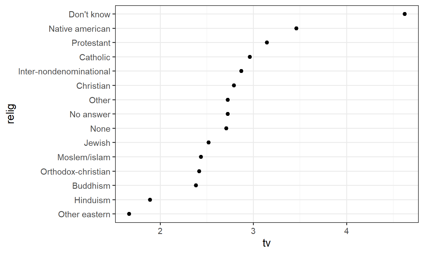

gss_cat |>
  mutate(partyid = fct_relevel(partyid, "Independent")) |>
  count(partyid)

## # A tibble: 10 × 2
##    partyid                n
##    <fct>              <int>
##  1 Independent         4119
##  2 No answer            154
##  3 Don't know             1
##  4 Other party          393
##  5 Strong republican   2314
##  6 Not str republican  3032
##  7 Ind,near rep        1791
##  8 Ind,near dem        2499
##  9 Not str democrat    3690
## 10 Strong democrat     3490

fct_infreq() then fct_rev() puts the most common level on the right of a bar chart.

4. Recode, collapse, lump

fct_recode() renames levels. Old name on the right. Drop a level with NULL = "old".

gss_cat |>
  mutate(partyid = fct_recode(
    partyid,
    "Rep, strong" = "Strong republican",
    "Rep, weak"   = "Not str republican",
    "Dem, weak"   = "Not str democrat",
    "Dem, strong" = "Strong democrat"
  )) |>
  count(partyid)

## # A tibble: 10 × 2
##    partyid          n
##    <fct>        <int>
##  1 No answer      154
##  2 Don't know       1
##  3 Other party    393
##  4 Rep, strong   2314
##  5 Rep, weak     3032
##  6 Ind,near rep  1791
##  7 Independent   4119
##  8 Ind,near dem  2499
##  9 Dem, weak     3690
## 10 Dem, strong   3490

fct_collapse() is recode for many-to-one. fct_lump() folds rare levels into Other. n keeps the most common; prop keeps levels above a share.

gss_cat |>
  mutate(partyid = fct_collapse(
    partyid,
    other = c("No answer", "Don't know", "Other party"),
    rep   = c("Strong republican", "Not str republican"),
    ind   = c("Ind,near rep", "Independent", "Ind,near dem"),
    dem   = c("Not str democrat", "Strong democrat")
  )) |>
  count(partyid)

## # A tibble: 4 × 2
##   partyid     n
##   <fct>   <int>
## 1 other     548
## 2 rep      5346
## 3 ind      8409
## 4 dem      7180

gss_cat |>
  mutate(relig = fct_lump(relig, n = 5)) |>
  count(relig)

## # A tibble: 6 × 2
##   relig          n
##   <fct>      <int>
## 1 Christian    689
## 2 None        3523
## 3 Jewish       388
## 4 Catholic    5124
## 5 Protestant 10846
## 6 Other        913

5. Add, drop, and missing levels

f <- factor(c("A", "B", "A"), levels = c("A", "B", "C"))
fct_drop(f)

## [1] A B A
## Levels: A B

g <- factor(c("A", "B"))
fct_expand(g, "C", "D")

## [1] A B
## Levels: A B C D

h <- factor(c("A", NA, "B"))
fct_explicit_na(h, na_level = "(Missing)")

## [1] A         (Missing) B        
## Levels: A B (Missing)

fct_drop() removes unused levels. fct_expand() adds empty ones. fct_explicit_na() turns NA into a real level so it appears in tables and plots. Filtering out rows does not drop the level; call fct_drop() after.

6. Practice

Use gss_cat.

1. Reorder partyid alphabetically.
2. Move rincome level "Not applicable" to the front.
3. Abbreviate marital with fct_recode().